%matplotlib inline

Transfer Learning for Computer Vision Tutorial

Author: Sasank Chilamkurthy <https://chsasank.github.io>_

In this tutorial, you will learn how to train a convolutional neural network for image classification using transfer learning. You can read more about the transfer learning at cs231n notes <https://cs231n.github.io/transfer-learning/>__

In practice, very few people train an entire Convolutional Network from scratch (with random initialization), because it is relatively rare to have a dataset of sufficient size. Instead, it is common to pretrain a ConvNet on a very large dataset (e.g. ImageNet, which contains 1.2 million images with 1000 categories), and then use the ConvNet either as an initialization or a fixed feature extractor for the task of interest.

These two major transfer learning scenarios look as follows:

• Finetuning the convnet: Instead of random initialization, we initialize the network with a pretrained network, like the one that is trained on imagenet 1000 dataset. Rest of the training looks as usual.

• ConvNet as fixed feature extractor: Here, we will freeze the weights for all of the network except that of the final fully connected layer. This last fully connected layer is replaced with a new one with random weights and only this layer is trained.

# License: BSD
# Author: Sasank Chilamkurthy

from __future__ import print_function, division

import torch
import torch.nn as nn
import torch.optim as optim
from torch.optim import lr_scheduler
import torch.backends.cudnn as cudnn
import numpy as np
import torchvision
from torchvision import datasets, models, transforms
import matplotlib.pyplot as plt
import time
import os
import copy

cudnn.benchmark = True
plt.ion()   # interactive mode

<contextlib.ExitStack at 0x7f718b80b520>

Load Data

We will use torchvision and torch.utils.data packages for loading the data.

The problem we’re going to solve today is to train a model to classify ants and bees. We have about 120 training images each for ants and bees. There are 75 validation images for each class. Usually, this is a very small dataset to generalize upon, if trained from scratch. Since we are using transfer learning, we should be able to generalize reasonably well.

This dataset is a very small subset of imagenet. The data was downloaded from https://download.pytorch.org/tutorial/hymenoptera_data.zip_ and extract it to the current directory.

# Unzip data
!mkdir -p data/hymenoptera_data
!unzip -o -q hymenoptera_data.zip -d data 

# Data augmentation and normalization for training
# Just normalization for validation
data_transforms = {
    'train': transforms.Compose([
        transforms.RandomResizedCrop(224),
        transforms.RandomHorizontalFlip(),
        transforms.ToTensor(),
        transforms.Normalize([0.485, 0.456, 0.406], [0.229, 0.224, 0.225])
    ]),
    'val': transforms.Compose([
        transforms.Resize(256),
        transforms.CenterCrop(224),
        transforms.ToTensor(),
        transforms.Normalize([0.485, 0.456, 0.406], [0.229, 0.224, 0.225])
    ]),
}

data_dir = 'data/hymenoptera_data'
image_datasets = {x: datasets.ImageFolder(os.path.join(data_dir, x),
                                          data_transforms[x])
                  for x in ['train', 'val']}
dataloaders = {x: torch.utils.data.DataLoader(image_datasets[x], batch_size=4,
                                             shuffle=True, num_workers=4)
              for x in ['train', 'val']}
dataset_sizes = {x: len(image_datasets[x]) for x in ['train', 'val']}
class_names = image_datasets['train'].classes

device = torch.device("cuda:0" if torch.cuda.is_available() else "cpu")

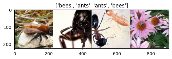
Visualize a few images

Let’s visualize a few training images so as to understand the data augmentations.

def imshow(inp, title=None):
    """Imshow for Tensor."""
    inp = inp.numpy().transpose((1, 2, 0))
    mean = np.array([0.485, 0.456, 0.406])
    std = np.array([0.229, 0.224, 0.225])
    inp = std * inp + mean
    inp = np.clip(inp, 0, 1)
    plt.imshow(inp)
    if title is not None:
        plt.title(title)
    plt.pause(0.001)  # pause a bit so that plots are updated


# Get a batch of training data
inputs, classes = next(iter(dataloaders['train']))

# Make a grid from batch
out = torchvision.utils.make_grid(inputs)

imshow(out, title=[class_names[x] for x in classes])

Training the model

Now, let’s write a general function to train a model. Here, we will illustrate:

• Scheduling the learning rate

• Saving the best model

In the following, parameter scheduler is an LR scheduler object from torch.optim.lr_scheduler.

def train_model(model, criterion, optimizer, scheduler, num_epochs=25):
    since = time.time()

    best_model_wts = copy.deepcopy(model.state_dict())
    best_acc = 0.0

    for epoch in range(num_epochs):
        print(f'Epoch {epoch}/{num_epochs - 1}')
        print('-' * 10)

        # Each epoch has a training and validation phase
        for phase in ['train', 'val']:
            if phase == 'train':
                model.train()  # Set model to training mode
            else:
                model.eval()   # Set model to evaluate mode

            running_loss = 0.0
            running_corrects = 0

            # Iterate over data.
            for inputs, labels in dataloaders[phase]:
                inputs = inputs.to(device)
                labels = labels.to(device)

                # zero the parameter gradients
                optimizer.zero_grad()

                # forward
                # track history if only in train
                with torch.set_grad_enabled(phase == 'train'):
                    outputs = model(inputs)
                    _, preds = torch.max(outputs, 1)
                    loss = criterion(outputs, labels)

                    # backward + optimize only if in training phase
                    if phase == 'train':
                        loss.backward()
                        optimizer.step()

                # statistics
                running_loss += loss.item() * inputs.size(0)
                running_corrects += torch.sum(preds == labels.data)
            if phase == 'train':
                scheduler.step()

            epoch_loss = running_loss / dataset_sizes[phase]
            epoch_acc = running_corrects.double() / dataset_sizes[phase]

            print(f'{phase} Loss: {epoch_loss:.4f} Acc: {epoch_acc:.4f}')

            # deep copy the model
            if phase == 'val' and epoch_acc > best_acc:
                best_acc = epoch_acc
                best_model_wts = copy.deepcopy(model.state_dict())

        print()

    time_elapsed = time.time() - since
    print(f'Training complete in {time_elapsed // 60:.0f}m {time_elapsed % 60:.0f}s')
    print(f'Best val Acc: {best_acc:4f}')

    # load best model weights
    model.load_state_dict(best_model_wts)
    return model

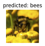
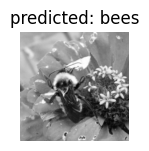
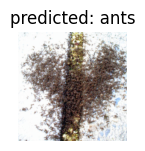
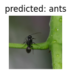
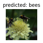
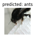
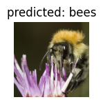
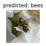
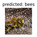
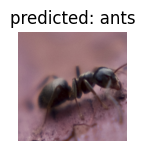
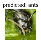
Visualizing the model predictions

Generic function to display predictions for a few images

def visualize_model(model, num_images=6):
    was_training = model.training
    model.eval()
    images_so_far = 0
    fig = plt.figure()

    with torch.no_grad():
        for i, (inputs, labels) in enumerate(dataloaders['val']):
            inputs = inputs.to(device)
            labels = labels.to(device)

            outputs = model(inputs)
            _, preds = torch.max(outputs, 1)

            for j in range(inputs.size()[0]):
                images_so_far += 1
                ax = plt.subplot(num_images//2, 2, images_so_far)
                ax.axis('off')
                ax.set_title(f'predicted: {class_names[preds[j]]}')
                imshow(inputs.cpu().data[j])

                if images_so_far == num_images:
                    model.train(mode=was_training)
                    return
        model.train(mode=was_training)

Finetuning the convnet

Load a pretrained model and reset final fully connected layer.

model_ft = models.resnet18(pretrained=True)
num_ftrs = model_ft.fc.in_features
# Here the size of each output sample is set to 2.
# Alternatively, it can be generalized to nn.Linear(num_ftrs, len(class_names)).
model_ft.fc = nn.Linear(num_ftrs, 2)

model_ft = model_ft.to(device)

criterion = nn.CrossEntropyLoss()

# Observe that all parameters are being optimized
optimizer_ft = optim.SGD(model_ft.parameters(), lr=0.001, momentum=0.9)

# Decay LR by a factor of 0.1 every 7 epochs
exp_lr_scheduler = lr_scheduler.StepLR(optimizer_ft, step_size=7, gamma=0.1)

/workspaces/artificial_intelligence/.venv/lib/python3.10/site-packages/torchvision/models/_utils.py:208: UserWarning: The parameter 'pretrained' is deprecated since 0.13 and may be removed in the future, please use 'weights' instead.
  warnings.warn(
/workspaces/artificial_intelligence/.venv/lib/python3.10/site-packages/torchvision/models/_utils.py:223: UserWarning: Arguments other than a weight enum or `None` for 'weights' are deprecated since 0.13 and may be removed in the future. The current behavior is equivalent to passing `weights=ResNet18_Weights.IMAGENET1K_V1`. You can also use `weights=ResNet18_Weights.DEFAULT` to get the most up-to-date weights.
  warnings.warn(msg)
Downloading: "https://download.pytorch.org/models/resnet18-f37072fd.pth" to /home/vscode/.cache/torch/hub/checkpoints/resnet18-f37072fd.pth

Train and evaluate

It should take around 15-25 min on CPU. On GPU though, it takes less than a minute.

model_ft = train_model(model_ft, criterion, optimizer_ft, exp_lr_scheduler,
                       num_epochs=25)

Epoch 0/24
----------
train Loss: 0.6682 Acc: 0.6844
val Loss: 0.4972 Acc: 0.8039

Epoch 1/24
----------
train Loss: 0.6931 Acc: 0.7254
val Loss: 0.2619 Acc: 0.9281

Epoch 2/24
----------
train Loss: 0.6481 Acc: 0.7828
val Loss: 0.2864 Acc: 0.8758

Epoch 3/24
----------
train Loss: 0.5984 Acc: 0.8156
val Loss: 0.6362 Acc: 0.7908

Epoch 4/24
----------
train Loss: 0.4897 Acc: 0.8115
val Loss: 0.4631 Acc: 0.8301

Epoch 5/24
----------
train Loss: 0.4897 Acc: 0.8197
val Loss: 0.3792 Acc: 0.8562

Epoch 6/24
----------
train Loss: 0.4491 Acc: 0.7951
val Loss: 0.3498 Acc: 0.8693

Epoch 7/24
----------
train Loss: 0.4476 Acc: 0.8156
val Loss: 0.3002 Acc: 0.8627

Epoch 8/24
----------
train Loss: 0.3146 Acc: 0.8689
val Loss: 0.2753 Acc: 0.8889

Epoch 9/24
----------
train Loss: 0.2530 Acc: 0.9139
val Loss: 0.2525 Acc: 0.8954

Epoch 10/24
----------
train Loss: 0.2522 Acc: 0.9098
val Loss: 0.2410 Acc: 0.9150

Epoch 11/24
----------
train Loss: 0.3417 Acc: 0.8484
val Loss: 0.2489 Acc: 0.9085

Epoch 12/24
----------
train Loss: 0.2227 Acc: 0.9098
val Loss: 0.2426 Acc: 0.9085

Epoch 13/24
----------
train Loss: 0.3280 Acc: 0.8607
val Loss: 0.2268 Acc: 0.9150

Epoch 14/24
----------
train Loss: 0.3335 Acc: 0.8648
val Loss: 0.2487 Acc: 0.9020

Epoch 15/24
----------
train Loss: 0.2828 Acc: 0.8730
val Loss: 0.2276 Acc: 0.9150

Epoch 16/24
----------
train Loss: 0.2447 Acc: 0.8975
val Loss: 0.2197 Acc: 0.9216

Epoch 17/24
----------
train Loss: 0.2392 Acc: 0.8893
val Loss: 0.2497 Acc: 0.9020

Epoch 18/24
----------
train Loss: 0.3230 Acc: 0.8770
val Loss: 0.2313 Acc: 0.9085

Epoch 19/24
----------
train Loss: 0.3141 Acc: 0.8566
val Loss: 0.2161 Acc: 0.9281

Epoch 20/24
----------
train Loss: 0.3094 Acc: 0.8730
val Loss: 0.2456 Acc: 0.9085

Epoch 21/24
----------
train Loss: 0.3657 Acc: 0.8566
val Loss: 0.2300 Acc: 0.9150

Epoch 22/24
----------
train Loss: 0.2825 Acc: 0.8770
val Loss: 0.2296 Acc: 0.9150

Epoch 23/24
----------
train Loss: 0.2966 Acc: 0.8648
val Loss: 0.2195 Acc: 0.9281

Epoch 24/24
----------
train Loss: 0.2631 Acc: 0.8893
val Loss: 0.2220 Acc: 0.9085

Training complete in 0m 37s
Best val Acc: 0.928105

visualize_model(model_ft)

ConvNet as fixed feature extractor

Here, we need to freeze all the network except the final layer. We need to set requires_grad = False to freeze the parameters so that the gradients are not computed in backward().

You can read more about this in the documentation here <https://pytorch.org/docs/notes/autograd.html#excluding-subgraphs-from-backward>__.

model_conv = torchvision.models.resnet18(pretrained=True)
for param in model_conv.parameters():
    param.requires_grad = False

# Parameters of newly constructed modules have requires_grad=True by default
num_ftrs = model_conv.fc.in_features
model_conv.fc = nn.Linear(num_ftrs, 2)

model_conv = model_conv.to(device)

criterion = nn.CrossEntropyLoss()

# Observe that only parameters of final layer are being optimized as
# opposed to before.
optimizer_conv = optim.SGD(model_conv.fc.parameters(), lr=0.001, momentum=0.9)

# Decay LR by a factor of 0.1 every 7 epochs
exp_lr_scheduler = lr_scheduler.StepLR(optimizer_conv, step_size=7, gamma=0.1)

Train and evaluate

On CPU this will take about half the time compared to previous scenario. This is expected as gradients don’t need to be computed for most of the network. However, forward does need to be computed.

model_conv = train_model(model_conv, criterion, optimizer_conv,
                         exp_lr_scheduler, num_epochs=25)

Epoch 0/24
----------
train Loss: 0.6031 Acc: 0.6680
val Loss: 0.2526 Acc: 0.9346

Epoch 1/24
----------
train Loss: 0.5132 Acc: 0.7254
val Loss: 0.2130 Acc: 0.9412

Epoch 2/24
----------
train Loss: 0.4905 Acc: 0.7787
val Loss: 0.2027 Acc: 0.9412

Epoch 3/24
----------
train Loss: 0.5901 Acc: 0.7336
val Loss: 0.1964 Acc: 0.9412

Epoch 4/24
----------
train Loss: 0.5100 Acc: 0.7951
val Loss: 0.3413 Acc: 0.8562

Epoch 5/24
----------
train Loss: 0.4256 Acc: 0.8033
val Loss: 0.1984 Acc: 0.9477

Epoch 6/24
----------
train Loss: 0.4232 Acc: 0.8279
val Loss: 0.1937 Acc: 0.9412

Epoch 7/24
----------
train Loss: 0.3542 Acc: 0.8115
val Loss: 0.1952 Acc: 0.9281

Epoch 8/24
----------
train Loss: 0.4106 Acc: 0.8320
val Loss: 0.1759 Acc: 0.9477

Epoch 9/24
----------
train Loss: 0.3410 Acc: 0.8279
val Loss: 0.1790 Acc: 0.9477

Epoch 10/24
----------
train Loss: 0.3573 Acc: 0.8238
val Loss: 0.1990 Acc: 0.9412

Epoch 11/24
----------
train Loss: 0.3382 Acc: 0.8525
val Loss: 0.1994 Acc: 0.9281

Epoch 12/24
----------
train Loss: 0.3315 Acc: 0.8484
val Loss: 0.1961 Acc: 0.9346

Epoch 13/24
----------
train Loss: 0.3014 Acc: 0.8730
val Loss: 0.2121 Acc: 0.9346

Epoch 14/24
----------
train Loss: 0.3267 Acc: 0.8648
val Loss: 0.2121 Acc: 0.9281

Epoch 15/24
----------
train Loss: 0.3681 Acc: 0.8238
val Loss: 0.2085 Acc: 0.9281

Epoch 16/24
----------
train Loss: 0.2891 Acc: 0.8689
val Loss: 0.2224 Acc: 0.9216

Epoch 17/24
----------
train Loss: 0.2871 Acc: 0.8811
val Loss: 0.2013 Acc: 0.9346

Epoch 18/24
----------
train Loss: 0.2311 Acc: 0.9139
val Loss: 0.1951 Acc: 0.9542

Epoch 19/24
----------
train Loss: 0.3362 Acc: 0.8320
val Loss: 0.2021 Acc: 0.9346

Epoch 20/24
----------
train Loss: 0.3685 Acc: 0.8443
val Loss: 0.2014 Acc: 0.9281

Epoch 21/24
----------
train Loss: 0.3464 Acc: 0.8607
val Loss: 0.2043 Acc: 0.9412

Epoch 22/24
----------
train Loss: 0.2885 Acc: 0.8811
val Loss: 0.1886 Acc: 0.9346

Epoch 23/24
----------
train Loss: 0.3048 Acc: 0.8730
val Loss: 0.1868 Acc: 0.9412

Epoch 24/24
----------
train Loss: 0.3638 Acc: 0.8361
val Loss: 0.2322 Acc: 0.9150

Training complete in 0m 23s
Best val Acc: 0.954248

visualize_model(model_conv)

plt.ioff()
plt.show()

Further Learning

If you would like to learn more about the applications of transfer learning, checkout our Quantized Transfer Learning for Computer Vision Tutorial <https://pytorch.org/tutorials/intermediate/quantized_transfer_learning_tutorial.html>_.