RNN-based Neural Machine Translation

These notes heavily borrowing from the CS229N 2019 set of notes on NMT.

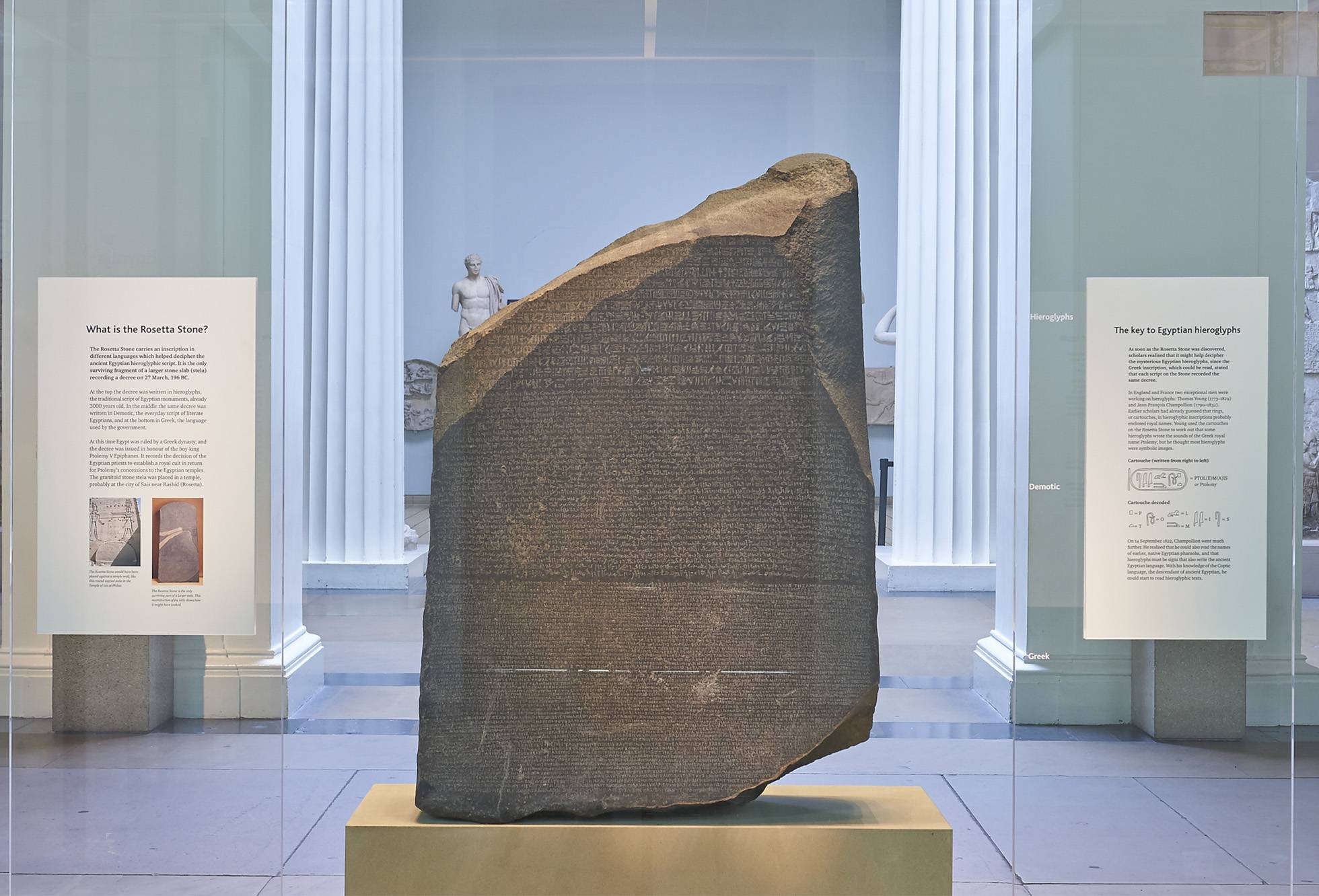Rosetta Stone at the British Museum - depicts the same text in Ancient Egyptian, Demotic and Ancient Greek.

Up to now we have seen how to generate word2vec embeddings and predict a single output e.g. the single most likely next word in a sentence given the past few. However, there’s a whole class of NLP tasks that rely on sequential output, or outputs that are sequences of potentially varying length. For example,

• Translation: taking a sentence in one language as input and outputting the same sentence in another language.

• Conversation: taking a statement or question as input and responding to it.

• Summarization: taking a large body of text as input and outputting a summary of it.

• Code Generation: Natural Language to formal language code (e.g. python)

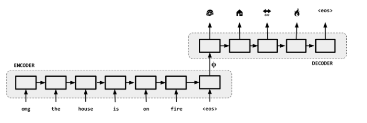Your smartphones translate the text you type in messaging applications to emojis and other symbols structured in such a way to convey the same meaning as the text.

Sequence-to-Sequence (Seq2Seq)

Sequence-to-sequence, or “Seq2Seq”, was first published in 2014. At a high level, a sequence-to-sequence model is an end-to-end model made up of two recurrent neural networks (LSTMs):

• an encoder, which takes the a source sequence as input and encodes it into a fixed-size “context vector” \(\phi\), and

• a decoder, which uses the context vector from above as a “seed” from which to generate an output sequence.

For this reason, Seq2Seq models are often referred to as encoder-decoder models as shown in the next figure.

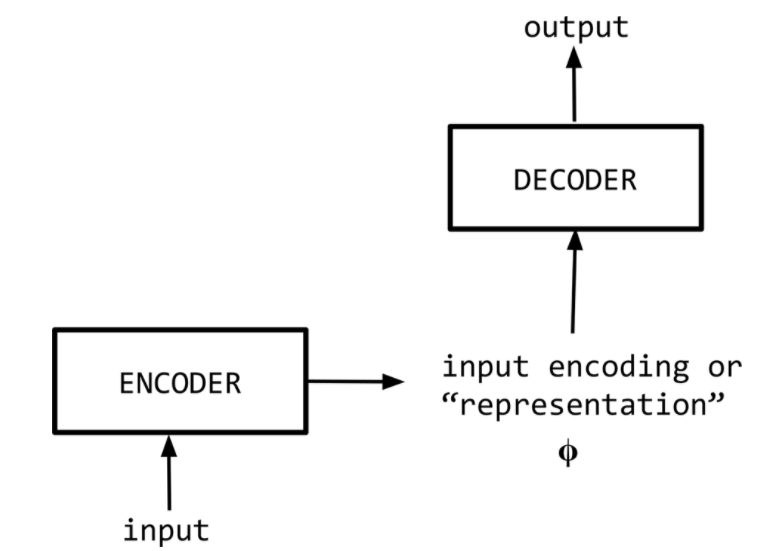Encoder-Decoder NMT Architecture ref

Encoder

The encoder network \(q\) reads the input sequence and generates a fixed-dimensional context vector \(\phi\) for the sequence. To do that we use an RNN that mathematically, it evolves its hidden state as follows:

\[\mathbf h_t = f(\mathbf x_t, \mathbf h_{t-1})\]

and \(f\) can be in e.g. any non-linear function such as an bidirectional RNN with a given depth. In the following we use the term RNN to refer to a gated RNN such as an LSTM.

The context vector is generated from the sequence of hidden states,

\[\mathbf \phi = q(\mathbf h_1, ..., \mathbf h_{Tx})\]

The bidirectional RNN is shown schematically below.

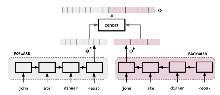Bidirectional RNNs used for representing each word in the context of the sentence

In this architecture, we read the input tokens one at a time to obtain the context vector \(\phi\). To allow the encoder to build a richer representation of the arbitrary-length input sequence, especially for difficult tasks like translation, the encoder usually consist of stacked (deep) RNNs: a series of RNN layers where each layer’s outputs are the input sequence to the next layer. In this architecture the final layer’s RNN hidden state will be used as \(\phi\).

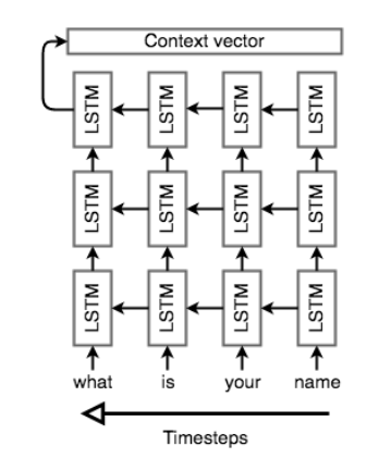Stacked LSTM Encoder (unrolled and showing the reverse direction only)

In addition, Seq2Seq encoders will often do something that initially look strange: they will process the input sequence in reverse. This is actually done on purpose with the idea being that the last thing that the encoder “sees” will roughly corresponds to the first thing that the model outputs; this makes it easier for the decoder to “get started” on the output.

Decoder

The decoder is “aware” of the target words that it’s generated so far and of the input. In fact it is an example of conditional language model because it conditions on the source sentence or its representation - the context \(\phi\).

The decoder directly calculates,

\[\mathbf{\hat y} = \arg \max_y p(\mathbf y | \mathbf \phi)\]

We can write this as:

\[\arg \max_y p(\mathbf y| \mathbf \phi) = \arg \max_y p(y_1, y_2, ..., y_{Ty} | \phi)\]

and then use the product rule of probability to decompose this to:

\[\arg \max_y p(y_{Ty} | y_1, ..., y_{Ty-1}, \mathbf \phi) \dots p(y_2|y_1, \mathbf \phi ) p(y_1| \mathbf \phi) \]

We can now write,

\[\mathbf{\hat y} = \arg \max_y p(\mathbf y | \mathbf \phi) = \arg \max \prod_{t=1}^{T_y} p(y_t | y_1, ..., y_{t-1}, \mathbf \phi) \]

In this equation \(p(y_t | y_1, ..., y_{t-1}, \mathbf \phi)\) is a probability distribution represented by a softmax across all all the words of the vocabulary.

We can use an RNN to model the conditional probabilities

\[LSTM = g(s_t, y_{t-1}, \phi ) = p(y_t | y_1, ..., y_{t-1}, \mathbf \phi) \]

To that end, we’ll keep the “stacked” LSTM architecture from the encoder, but we’ll initialize the hidden state of our first layer with the context vector. Once the decoder is set up with its context, we’ll pass in a special token to signify the start of output generation; in literature, this is usually an token appended to the end of the input (there’s also one at the end of the output). Then, we’ll run all stacked layers of LSTM, one after the other, following at the end with a softmax on the final layer’s output that can tell us the most probable output word.

Both the encoder and decoder are trained at the same time, so that they both learn the same context vector representation as shown next.

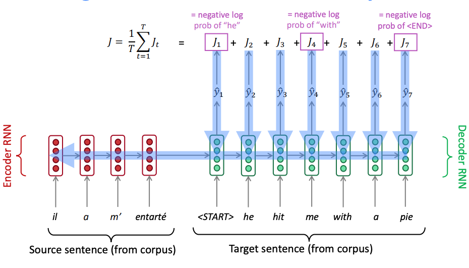Seq2Seq Training - backpropagation is end to end.

To help training, we apply teacher forcing wherein the input at each time step to the decoder is the ground truth. During inference just like in the language model we input the predicted output from the previous time step.

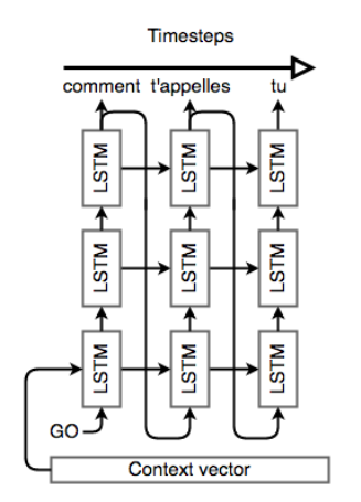LSTM Decoder (unrolled). The decoder is a language model that’s “aware” of the words that it’s generated so far and of the input.

Once we have the output sequence, we use the same learning strategy as usual. We define a loss, the cross entropy on the prediction sequence, and we minimize it with a gradient descent algorithm and back-propagation.

Note that the \(\arg \max\) we apply at each step on the softmax output results in some instances in suboptimal translations. Beam search, a method that is rooted in maximum likelihood sequence estimation and the Viterbi algorithm, maintains a small number (e.g. 3-10) of the top likely sentences called the beam width , as opposed to the most likely sentence, and tries to extend them by one word at each step.