Temporal Difference (TD) Prediction

If one had to identify one idea as central and novel to reinforcement learning, it would undoubtedly be temporal-difference(TD) learning. TD learning is a combination of Monte Carlo ideas and dynamic programming (DP) ideas.

• Like Monte Carlo methods, TD methods can learn directly from raw experience without a model of the environment’s dynamics.

• Like DP, TD methods update estimates based in part on other learned estimates, without waiting for a final outcome.

In TD, instead of getting an estimated value function at the end of multiple episodes, we can use the incremental mean approximation to update the value function after each step.

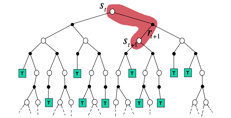
Backup tree for value iteration with the TD approach. TD samples a single step ahead as shown with red.

Going back to the example of crossing the room optimally, we take one step towards the goal and the we bootstrap the value function of the state we were in from an estimated return for the remaining trajectory. We repeat this as we go along effectively adjusting the value estimate of the starting state from the true returns we have experienced up to now, gradually grounding the whole estimate as we approach the goal.

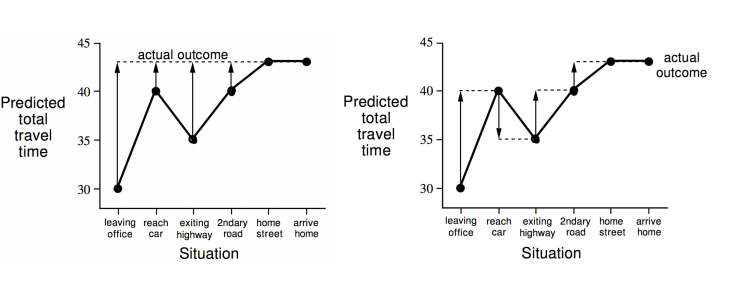
Two value approximation methods: MC (left), TD (right) as converging in their predictions of the value of each of the states in the x-axis. The example is from a hypothetical commute from office back home. In MC you have to wait until the episode ended (reach the goal) to update the value function at each state of the trajectory. In contrast, TD updates the value function at each state based on the estimates of the total travel time. The goal state is “arrive home”, while the reward function is time.

As you can notice in the figure above the solid arrows in the MC case, adjust the predicted value of each state to the actual return while in the TD case the value prediction happens every step in the way. We call TD for this reason an online learning scheme. Another characteristic of TD is that it does not depend on reaching the goal, it continuously learns. MC does depend on the goal and therefore is episodic. This is important in many mission critical applications eg self-driving cars where you dont wait to “crash” to apply corrections to your state value based on what you experienced.

Mathematically, instead of using the true return, \(G_t\), something that it is possible in the MC as we are trully experiencing the world along a trajectory, TD uses a (biased) estimated return called the TD target: \( R_{t+1} + \gamma V(S_{t+1})\) approximating the value function as:

\[ V(S_t) = V(S_t) + \alpha \left( R_{t+1} + \gamma V(S_{t+1}) - V(S_t) \right)\]

The difference below is called the TD approximation error,

\[\delta_t = R_{t+1} + \gamma (V(S_{t+1}) - V(S_t))\]

The TD(\(\lambda\))

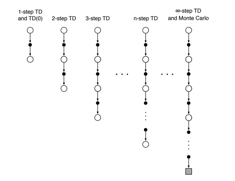
The TD approach of the previous section, can be extended to multiple steps. Instead of a single look ahead step we can take multiple successive look ahead steps (n), we will call this TD(n) for now, and at the end of the n-th step, we use the value function at that state to backup and get the value function at the state where we started. The trees below are indicative of the process.

Effectively after n-steps our return will be:

\[G_{t:t+n} = R_{t+1} + \gamma R_{t+2} + \gamma^2 R_{t+3} + ... + \gamma^{n-1}R_{t+n} + \gamma^{n} V_{t+n-1}(S_{t+n})\]

and the TD(n) learning equation becomes

\[ V(S_t) = V(S_t) + \alpha \left( G_{t:t+n} - V(S_t) \right) \]

We now define the so called \(\lambda\)-return that combines all n-step returns \(G_{t:t+n}\) via the geometric weighting function shown below:

\[G_t^{(\lambda)} = (1-\lambda) \sum_{n=1}^{T-(t+1)} \lambda^{n-1} G_{t:t+n} + (1-\lambda) \lambda^{T-(t+1)}G_t\]

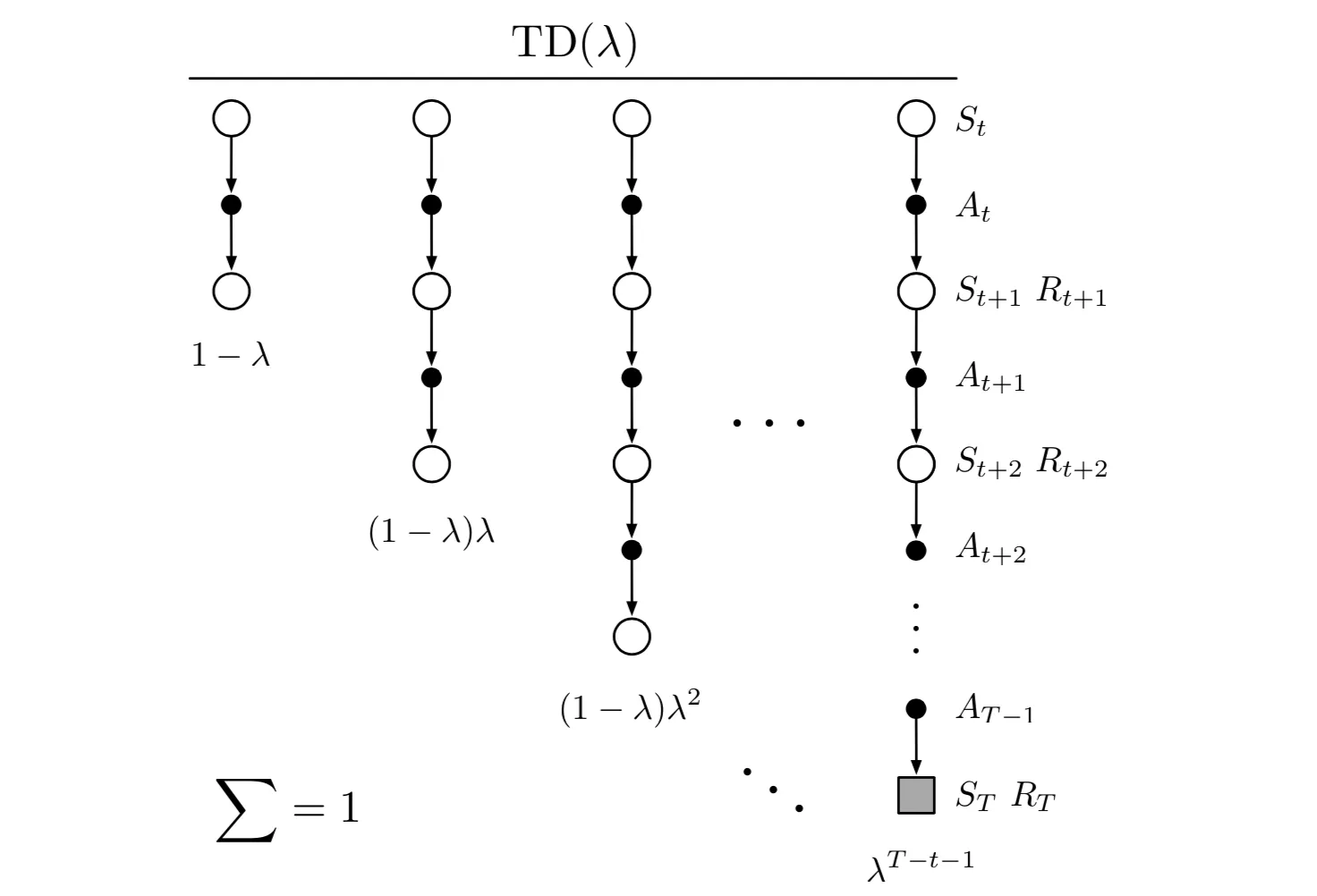
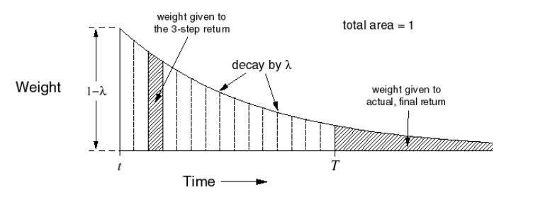
\(\lambda\) weighting function for TD(\(\lambda\))

the TD(n) learning equation becomes

\[ V(S_t) = V(S_t) + \alpha \left( G^\lambda_t - V(S_t) \right) \]

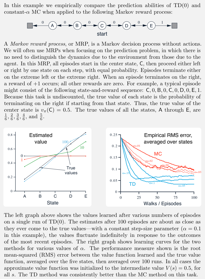
When \(\lambda=0\) we get TD(0) learning (the 1-step TD), while when \(\lambda=1\) we get learning that is roughly equivalent to MC. Certainly it is convenient to learn one guess from the next, without waiting for an actual outcome, but can we still guarantee convergence to the correct answer? Happily, the answer is yes as shown in the figure above. For any fixed policy \(π\), TD(0) has been proved to converge to \(v_π\), in the mean for a constant step-size parameter if it is sufficiently small. However in terms of data efficiency there is no clear winner at this point. It is instructive to see the difference between MC and TD approaches in the following example.