Attention in RNN-based NMT

When you hear the sentence “the soccer ball is on the field,” you don’t assign the same importance to all 7 words. You primarily take note of the words “ball” “on,” and “field” since those are the words that are most descriptive to you.

Using the final RNN hidden state as the single context vector sequence-to-sequence models cannot differentiate between significant and less significant words. Moreover, different parts of the output need to consider different parts of the input as “important.”

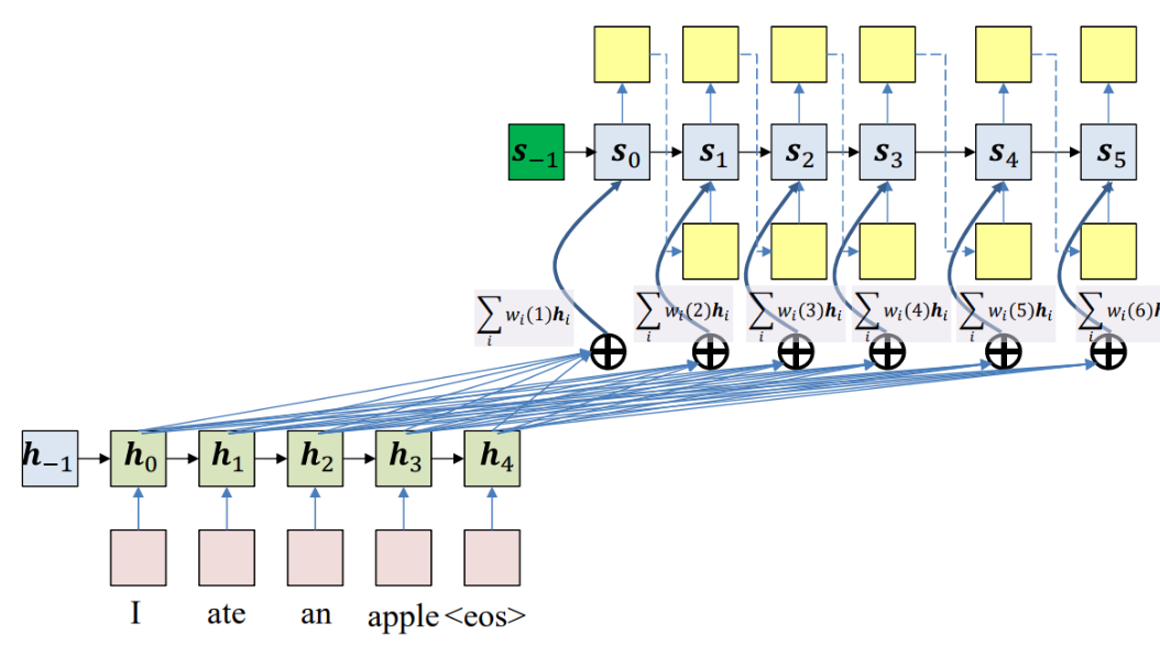
To address this issue we can simply introduce skip connections - similarly to the ResNet architecture - to the RNN decoder. We can decorate each skip connection with a weight that is learned during training. In the figure below you can see the encoder hidden states combined via a weighted sum with the decoder hidden states.

Important

Notice that if the set of weights that the decoder uses to combine the encoder hidden states is the same for all decoder hidden states, this will not solve the problem as the decoder may need to focus on different parts of the input at different time steps. We therefore make the weights dynamic and dependent on the decoder hidden state.

The attention mechanism will calculate these weights: it will make use of this observation by providing the decoder network with a look at the entire input sequence at every decoding step and having the decoder decide what input words are important at any point in time and effectively making the context dependent on decoder time step.

The current decoder state can be thought as a query while the encoder states \(h_i\) can be thought as keys and the contents of such hidden state as values. The attention weights are computed by comparing the query against each of the keys and passing the results via a softmax. The values are then used to create a weighted sum of the encoder hidden states to obtain the new decoder state ie. a vector that incorporates all the encoder hidden states. Note that keys and values are the same in this description but they can also be different.

1. During encoding the output of bidirectional LSTM encoder can provide the contextual representation of each input word \(x_i\). Let the encoder hidden vectors be denoted as \(h_1, ..., h_{Tx}\) where \(Tx\) is the length of the input sentence.

2. During decoding we compute the RNN decoder hidden states \(s_t\) using a recursive relationship,

\[s_t = g(s_{t-1}, y_{t-1}, \phi_t)\]

where \(s_{t-1}\) is the previous hidden state, \(y_{t-1}\) is the word at the previous step and \(\phi_t\) is the context vector that captures the context from the original sentence that is relevant to the decoder at time \(t\).

The \(\phi_t\) is computed with the help of a small neural network called attention layer, which is trained jointly with the rest of the Encoder–Decoder model. This model, is also known as allignment model since it alligns the decoder step and the relevant context for that step, is illustrated on the right hand side of the figure above.

Example

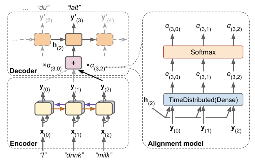Attention mechanism in NMT. Instead of just sending the encoder’s final hidden state to the decoder (which is still done, although it is not shown in the figure), we now send all of its outputs to the decoder. At each time step, the decoder’s memory cell computes a weighted sum of all these encoder outputs: this determines which words it will focus on at this step. The weight \(a_t(i)\) is the weight of the ith encoder output at the t-th decoder time step. For example, if the weight \(α_3(2)\) is much larger than the weights \(α_3(0)\) and \(α_3(1)\), then the decoder will pay much more attention to word number 2 (“milk”) than to the other two words, at least at this time step.

It starts with a time-distributed Dense layer with a single neuron, which receives as input all the encoder outputs, concatenated with the decoder’s previous hidden state (e.g., \(\mathbf h_2\)). This layer outputs a score (or energy) for each encoder output that measures how well each output is aligned with the decoder’s previous hidden state.

More specifically the \(\phi_t\) is computed as follows:

1. For each hidden state from the source sentence \(h_i\) (key), \(i\) is the sequence index of the encoder hidden state, we compute a score

\[e_{t,i} = \mathtt{scoring}(h_i, s_{t−1})\]

where \(\mathtt{scoring}\) is any function with values in \(\mathbb R\) - see below for choices of scoring functions. The other argument in the scoring function is the previous decoder hidden state \(s_{t-1}\) (query).

2. The score values are normalized using a softmax layer to produce the attention weight vector \(\mathbf α_t\). All the weights for a given decoder time step add up to 1.

\[\mathbf a_t = \mathtt{softmax}(\mathbf e_{t})\]

3. The context vector \(\phi_t\) is then the attention weighted average of the hidden state vectors (values) from the original sentence.

\[ \phi_t = \sum_i \alpha_{t,i}h_i\]

Intuitively, this vector captures the relevant contextual information from the original sentence for the t-th step of the decoder.

The two figures below showcase what it happening in two different time instances of an example french to english translation. Notice how the attention weights calculated via the softmax that puts a lot of emphasis to the highest score vary. In time zone one the attention mechanism weighs on the pronoun and in time step 6 it weighs on the object.

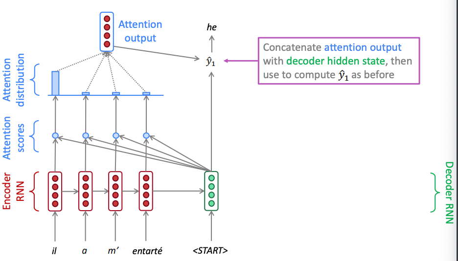Attention in seq2seq neural machine translation - time step 1

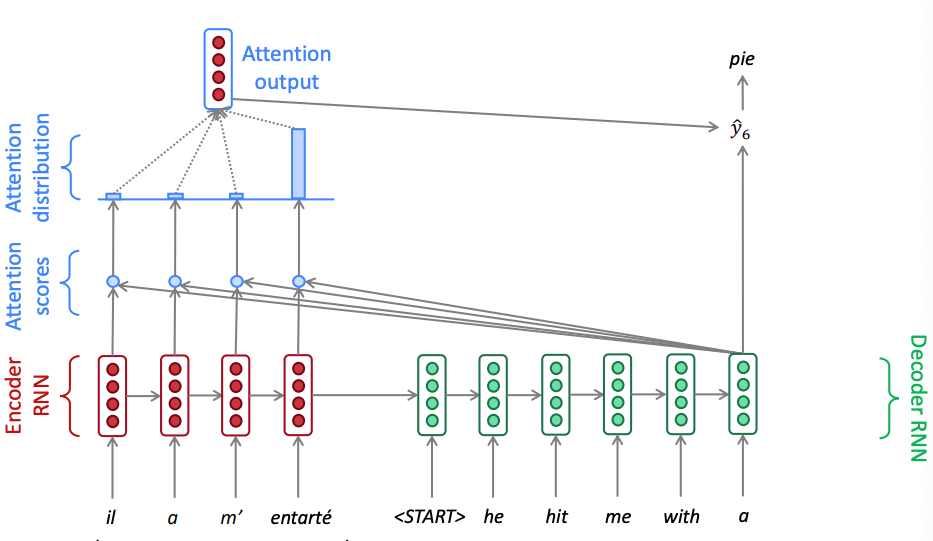Attention in seq2seq neural machine translation - time step 6

Scoring functions

There are multiple attention mechanisms and typically the Bahdanau attention is often quoted. It implements a fully connected neural network in the scoring function that adds the projected encoder \(W h_i\) and decoder hidden states \(U s_{t-1}\) (additive attention):

\[e_{t,i} = \mathtt{scoring}(s_{t−1}, h_i) = \mathbf v^T \tanh(W h_i + U s_{t-1})\]

During the decoding step it concatenates the encoder output with the decoder’s previous hidden state and this is why sometimes is also called concatenative attention.

There is alsp multiplicative attention that uses a dot product between encoder and decoder hidden states and there is also a Luong attention that uses a linear unit for scoring. Note that in this case we use the current decoder hidden state.

\[e_{t,i} = \mathtt{scoring}(s_t, h_i) = \mathbf s_{t}^T W h_i\]

Notice that the there is no concatenation during the decoding step. In the workshop we will use the multiplicative attention mechanism.