Bellman Optimality Backup

Now that we can calculate the value functions efficiently via the Bellman expectation recursions, we can now solve the MDP which requires maximize either of the two functions over all possible policies. The optimal state-value function and optimal action-value function are given by definition,

\[v_*(s) = \max_\pi v_\pi(s)\]

\[q_*(s,a) = \max_\pi q_\pi(s,a)\]

The \(v_*(s)\) is the best possible value (expected return) we can get starting from state \(s\). The \(q_*(s,a)\) is the best value (expected return) starting at state \(s\) and taking an action \(a\). In other words we can now obtain the optimal policy by maximizing over \(q_*(s,a)\) - mathematically this can be expressed as,

\[\begin{split}\pi_*(a|s) = \begin{cases}1 & \text{if }\ a = \arg \max_{a \in \mathcal A} q_*(s,a), \\ 0 & \text{otherwise}\end{cases}\end{split}\]

So the problem now becomes how to calculate the optimal value functions. We return to the tree structures that helped us understand the interdependencies between the two and this time we look at the optimal equivalents.

Actions can be taken from that state \(s\) according to the policy \(\pi_*\)

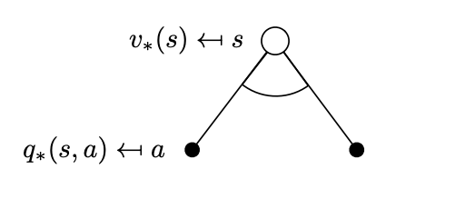
Following similar reasoning as in the Bellman expectation equation where we calculated the value of state \(s\) as an average of the values that can be claimed by taking all possible actions, now we simply replace the average with the max.

\[v_*(s) = \max_a q_*(s,a)\]

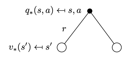
Successor states that can be reached from state \(s\) if the agent selects action \(a\). \(R_{t+1}=r\) we denote the instantaneous reward for each of the possibilities.

Similarly, we can express \(q_*(s,a)\) as a function of \(v_*(s)\) by looking at the corresponding tree above.

\[q_*(s,a) = \mathcal R_s^a + \gamma \sum_{s^\prime \in \mathcal S} \mathcal{P}^a_{ss^\prime} v_*(s^\prime)\]

Notice that there is no \(\max\) is this expression as we have no control on the successor state - that is something the environment controls. So all we can do is average.

Now we can similarly attempt to create a recursion that will lead to the Bellman optimality backup equations that effectively solve the MDP, by expanding the trees above.

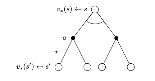
Tree that represents the optimal state-value function after a two-step look ahead.

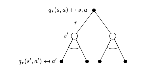
Tree that represents the optimal action-value function after a two-step look ahead.

Note

Bellman Optimality Backup

\[v_*(s) = \max_a \left( \mathcal R_s^a + \gamma \sum_{s^\prime \in \mathcal S} \mathcal{P}^a_{ss^\prime} v_*(s^\prime) \right)\]

\[q_*(s,a) = \mathcal R_s^a + \gamma \sum_{s^\prime \in \mathcal S} \mathcal{P}^a_{ss^\prime} \max_{a^\prime} q_*(s^\prime,a^\prime)\]

These equations due to the \(\max\) operator are non-linear and can be solved to obtain the MDP solution aka \(q_*(s,a)\) iteratively via a number of methods: policy iteration, value iteration, Q-learning, SARSA. We will see some of these methods in detail in later chapters. The key advantage in the Bellman optimality equations is efficiency:

1. They recursively decompose the problem into two sub-problems: the subproblem of the next step and the optimal value function in all subsequent steps of the trajectory.

2. They cache the optimal value functions to the sub-problems and by doing so we can reuse them as needed.

Since the Bellman equations allow us to decompose recursively the problem into sub-problems, they in fact implement a general and exact approach called dynamic programming that results into an optimal policy. We examine the computational aspects of such approach in a separate section.

References

The notes above are based on David Silver’s tutorial videos linked earlier. The video below is also an excellent introduction to MDP problems and includes python code that solves a simple MDP problem.