Single-head self-attention

Scaled dot-product self-attention

In the simple attention mechanism, the attention weights are computed deterministically from the input context. We call the combination of context-free embedding (eg word2vec) and positional embedding, the input embedding. What we would like to do is to Given the input embedding, the output embedding has no information about the data distribution that the input token is part of outside the context.

Lets look at the grammatical structure of the following sentences:

1. “I love bears”

   • Subject: I

   • Verb: love

   • Object: bears

2. “She bears the pain”

   • Subject: She

   • Verb: bears

   • Object: the pain

3. “Bears won the game”

   • Subject: Bears

   • Verb: won

   • Object: the game

Each sentence above follows a subject-verb-object structure, where the subject performs the action expressed by the verb on the object. You can notice that bears plays a different function in each sentence: as an object, as a verb, and as a subject. In addition, we have other and more complicated language patterns, such as this:

4. “The hiking trail led us through bear country.”

   • Subject: “The hiking trail”

   • Verb: “led”

   • Object: “us”

   • Prepositional Phrase: “through bear country”

   • Preposition: “through”

   • Object of the Preposition: “bear country”

     • Noun: “country”

     • Adjective: “bear” (modifying “country”)

Here, “bear” serves as an adjective describing the type of country.

The central question that one can pose now is this: Since the location of the token seems highly correlated with its function, as captured by the language patterns above, how can we help the embedding mapping become location aware and function aware ?

Linear transformation of the input embeddings

This is done by projecting the input embeddings using a projection matrix \(W\) obtaining a new coordinate system whose axes can be associated with object, verb, subject, adjective etc. The semantic meaning of such new coordinate system is not necessary to be explicitly defined but it helps understand what this projection may achieve.

We define three such trainable matrices \(W^q, W^k, W^v\) and ask each token (or equivalently the matrix \(X\)) to project itself to the three different spaces.

\[Q = XW^q\]

\[K = XW^k\]

\[V = XW^v\]

where \(X\) is the input embedding matrix of size \(T \times d\) where \(T\) is the input sequence length and \(d\) is the embedding dimension. \(Q, K, V\) are the query, keys and values respectively and the dimensions of the \(W^q, W^k, W^v\) matrices are \(d \times d_q, d \times d_k, d \times d_v\) respectively. Queries and keys occupy typically the same dimensional space (\(d_k\)).

Each token is undertaking three roles, lets focus here on the first two:

In a query role the current token effectively seeks to find other functions eg ‘adjective’ In a key role the current token effectively expresses its own function eg ‘noun’.

For example: ‘I am key=noun’ and I am seeking for a earlier query=adjective’.

The premise that that after training, the attention mechanism will be able to reveal the keys of the input context that can best respond to the query.. Notice also something not obvious.

Let us now recall what we saw already during the word2vec construction: we trained a network that will take one-hot vectors of semantically similar tokens that were orthonormal and projected them to vectors that are close to each other in the embedding space. So we have seen evidence that a projection with proper weights can cause all sorts of interesting mappings to happen from a large dimensional space to a lower space. By analogy, the multiplication of the matrix \(W^q\) with the input token embedding will create a vector (a point) in the d_k dimensional space that will represent the query. Similarly the multiplication of the matrix \(W^k\) with each and every input token embedding will create vectors (a point) in the d_k dimensional space that will represent the keys. After training the keys that can best respond to the query will end up close to it.

Computation of the attention scores

Lets see an example of the projection of the input embeddings to the query and key spaces for the input context.
Given matrices \( X \) and \( W^{(q)} \) (the key parameter matrix is analogous) where:

\[\begin{split} X = \begin{bmatrix} x_{1,1} & x_{1,2} & x_{1,3} & x_{1,4} & x_{1,5} & x_{1,6} & x_{1,7} & x_{1,8} \\ x_{2,1} & x_{2,2} & x_{2,3} & x_{2,4} & x_{2,5} & x_{2,6} & x_{2,7} & x_{2,8} \\ \vdots & \vdots & \vdots & \vdots & \vdots & \vdots & \vdots & \vdots \\ x_{16,1} & x_{16,2} & x_{16,3} & x_{16,4} & x_{16,5} & x_{16,6} & x_{16,7} & x_{16,8} \end{bmatrix} \end{split}\]

\[\begin{split} W^{(q)} = \begin{bmatrix} w_{1,1} & w_{1,2} & w_{1,3} & w_{1,4} \\ w_{2,1} & w_{2,2} & w_{2,3} & w_{2,4} \\ \vdots & \vdots & \vdots & \vdots \\ w_{8,1} & w_{8,2} & w_{8,3} & w_{8,4} \end{bmatrix} \end{split}\]

The resulting matrix \( Q \), where \( Q = X \times W^{(q)} \), will have dimensions \( 16 \times 8 \). Each element \( q_{i,j} \) of \( Q \) is computed as:

\[ q_{i,j} = x_{i,1} \cdot w_{1,j} + x_{i,2} \cdot w_{2,j} + x_{i,3} \cdot w_{3,j} + x_{i,4} \cdot w_{4,j} \]

Notice something not obvious earlier: the matrix \(W^{(q)}\) allows to weigh differently some features of the input embedding (across the \(d\) dimensions) than others when it calculates the query and key vectors.

Lets now proceed with the evolved dot product that now is done at the query-key \(d_q = d_k\) space.

“The hiking trail led us through bear country.” where \(T=8\)

\[\begin{split} \begin{array}{cccccccc} & q_1 & q_2 & q_3 & q_4 & q_5 & q_6 & q_7 & q_8 \\ k_1 & {q_1^T k_1} & {q_2^T k_1} & {q_3^T k_1} & {q_4^T k_1} & {q_5^T k_1} & {q_6^T k_1} & {q_7^T k_1} & {q_8^T k_1} \\ k_2 & {q_1^T k_2} & {q_2^T k_2} & {q_3^T k_2} & {q_4^T k_2} & {q_5^T k_2} & {q_6^T k_2} & {q_7^T k_2} & {q_8^T k_2} \\ k_3 & {q_1^T k_3} & {q_2^T k_3} & {q_3^T k_3} & {q_4^T k_3} & {q_5^T k_3} & {q_6^T k_3} & {q_7^T k_3} & {q_8^T k_3} \\ k_4 & {q_1^T k_4} & {q_2^T k_4} & {q_3^T k_4} & {q_4^T k_4} & {q_5^T k_4} & {q_6^T k_4} & {q_7^T k_4} & {q_8^T k_4} \\ k_5 & {q_1^T k_5} & {q_2^T k_5} & {q_3^T k_5} & {q_4^T k_5} & {q_5^T k_5} & {q_6^T k_5} & {q_7^T k_5} & {q_8^T k_5} \\ k_6 & {q_1^T k_6} & {q_2^T k_6} & {q_3^T k_6} & {q_4^T k_6} & {q_5^T k_6} & {q_6^T k_6} & {q_7^T k_6} & {q_8^T k_6} \\ k_7 & {q_1^T k_7} & {q_2^T k_7} & {q_3^T k_7} & {q_4^T k_7} & {q_5^T k_7} & {q_6^T k_7} & {q_7^T k_7} & {q_8^T k_7} \\ k_8 & {q_1^T k_8} & {q_2^T k_8} & {q_3^T k_8} & {q_4^T k_8} & {q_5^T k_8} & {q_6^T k_8} & {q_7^T k_8} & {q_8^T k_8} \\ \end{array} \end{split}\]

Now that we have projected the tokens in their new space we can form the generalized dot product

\[(W^qx_i)^TW^kx_j = x_i^T (W^q)^TW^kx_j=x_i^TWx_j\]

Geometrically you can visualize this as shown below:

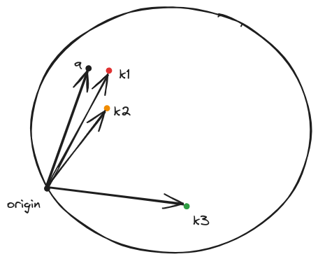After training the keys that can the most to change the query will end up close to it. The actual change of the query is done by the values.

The scores are then given in matrix form by:

\[S = QK^T\]

Scaling

We divide the scores by the square root of the dimension of the key vector (\(d_k\)). This is done in to prevent the softmax from saturating on the higher attention score elements and severely attenuating the attention weights that correspond to the lower attention scores.

We can do an experiment to see the behavior of softmax.

import numpy as np

# Creating an 8-element numpy vector with random gaussian values
vector = np.random.randn(8)

# Softmax function
def softmax(x):
    e_x = np.exp(x - np.max(x)) # Stability improvement by subtracting the max
    return e_x / e_x.sum()

# Applying softmax to the vector
softmax_vector = softmax(vector)
softmax_vector

Lets plot the two results - the first case is when for the original vector and the second case is when the original vector is element-wise multiplied by 100.

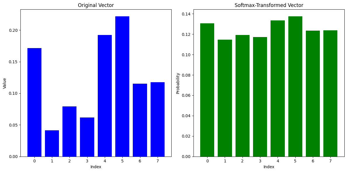
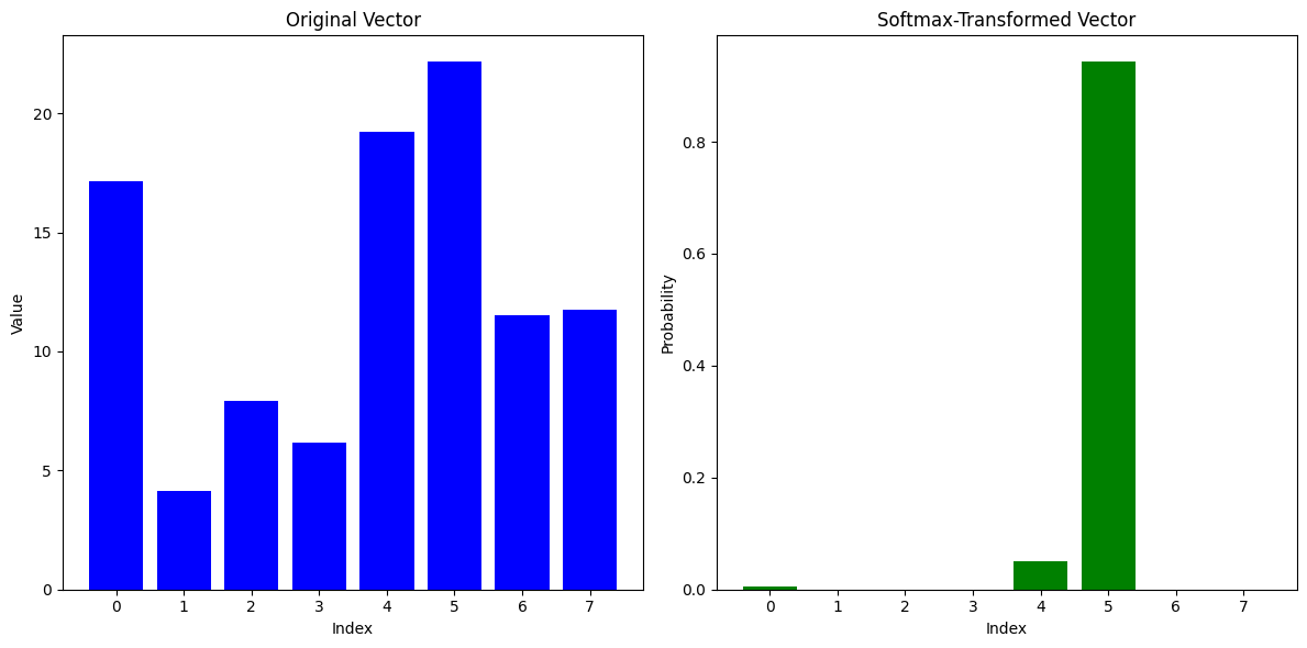
Multiply the attention scores by 100 and then pass them through a softmax. You will see that the softmax will output a vector of values that are either very close to 0 or 1.

The division by the \(\sqrt{d_k}\) prevents this behavior.

The code for the scaled dot product attention is shown below.

def scaled_dot_product_attention(query, key, value):
    dim_k = query.size(-1)
    scores = torch.bmm(query, key.transpose(1, 2)) / sqrt(dim_k)
    weights = F.softmax(scores, dim=-1)
    return torch.bmm(weights, value)

Masking

When we decode we do not want to use the attention scores of the future tokens since we dont want to train the tranformer using ground truth that will simply wont be available during inference.

To prevent this from happening we mask the attention scores of the future tokens by setting them to \(-\infty\) before passing them through the softmax. This will cause the softmax to output a vector of values that are very close to 0 for the future tokens.

\[\begin{split} \begin{array}{cccccccc} & q_1 & q_2 & q_3 & q_4 & q_5 & q_6 & q_7 & q_8 \\ k_1 & {q_1^T k_1} & {q_2^T k_1} & {q_3^T k_1} & {q_4^T k_1} & {q_5^T k_1} & {q_6^T k_1} & {q_7^T k_1} & {q_8^T k_1} \\ k_2 & -\infty & {q_2^T k_2} & {q_3^T k_2} & {q_4^T k_2} & {q_5^T k_2} & {q_6^T k_2} & {q_7^T k_2} & {q_8^T k_2} \\ k_3 & -\infty & -\infty & {q_3^T k_3} & {q_4^T k_3} & {q_5^T k_3} & {q_6^T k_3} & {q_7^T k_3} & {q_8^T k_3} \\ k_4 & -\infty & -\infty & -\infty & {q_4^T k_4} & {q_5^T k_4} & {q_6^T k_4} & {q_7^T k_4} & {q_8^T k_4} \\ k_5 & -\infty & -\infty & -\infty & -\infty & {q_5^T k_5} & {q_6^T k_5} & {q_7^T k_5} & {q_8^T k_5} \\ k_6 & -\infty & -\infty & -\infty & {q_4^T k_6} & {q_5^T k_6} & {q_6^T k_6} & {q_7^T k_6} & {q_8^T k_6} \\ k_7 & -\infty & -\infty & -\infty & -\infty & -\infty & -\infty & {q_7^T k_7} & {q_8^T k_7} \\ k_8 & -\infty & -\infty & -\infty & -\infty & -\infty & -\infty & -\infty & {q_8^T k_8} \\ \end{array} \end{split}\]

Softmax

The dot-product terms will be positive or negative numbers and as also in the case of the simpler version of the attention mechanism, we will pass them through a softmax function column-wise to obtain the attention weights \(\alpha_{ij}\) for each of the tokens.

Weighting the values

We then use the attention weights to create a weighted sum of each of the values to obtain the output embedding.

\[\hat v_i = \sum_{j=1}^T \alpha_{ij} v_j\]

where \(\alpha_{ij}\) is the attention weight of the \(j-th\) token of the input sequence for the \(i-th\) value of the input sequence of length T.

Why purpose the values play though and why the \(W^v\) matrix ?

The values are the actual information that the input token will use to update its embedding. The \(W^v\) matrix is used to project the input tokens to values (points) in a \(d_v\) dimensional space. There is no reason to make the dimensionality of the value space the same as the dimensionality of the key space but typically they are the same. We use the value projection (\(V\)) as a way to decouple the determination of the attention weights from the actual adjustment of their specific embeddings.

As an example, in the context “The hiking trail led us through bear country”, if the key represents the adjective of an input token that responded to a noun query, the value will represent the specific adjective (bear) that adjusts the specific noun (country) and makes it a bear country vector.

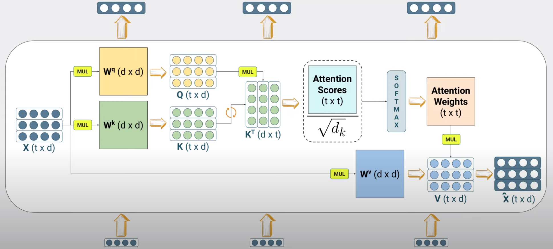Note that masking is not shown in this figure. Also vector subspaces maintain the same dimensions throughout.

Closing, the overall equation for the scaled self-attention can be formulated as:

\[\hat X = \mathtt{Attention}(Q, K, V) = \mathtt{softmax}(\frac{QK^T}{\sqrt{d_k}})V\]

and the output has dimension \(c \times d_v\) where \(c\) is the number of tokens in the input sequence and \(d_v\) is the dimension of the value vectors.

The dimensions of the tensors can also be extended to accommodate the batch dimension.

Dense Layers and Self-Attention

Its worthwhile highlighting the difference between a dense layer and the self-attention mechanism. In a dense layer, if the layer learns to apply eg a very small weight at the input, it does so for all data that are fed into the layer. In the self-attention mechanism if one of the attention weights is for example very small, this is purely due to the specific data being present.

Example

An example of the output of the scaled dot-product self-attention is shown below using the bertviz library.

from bertviz import head_view
from transformers import AutoModel

model = AutoModel.from_pretrained(model_ckpt, output_attentions=True)

sentence_a = "time flies like an arrow"
sentence_b = "fruit flies like a banana"

viz_inputs = tokenizer(sentence_a, sentence_b, return_tensors='pt')
attention = model(**viz_inputs).attentions
sentence_b_start = (viz_inputs.token_type_ids == 0).sum(dim=1)
tokens = tokenizer.convert_ids_to_tokens(viz_inputs.input_ids[0])

head_view(attention, tokens, sentence_b_start, heads=[8])

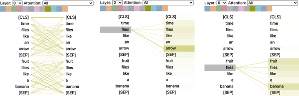
This visualization shows the attention weights as lines connecting the token whose embedding is getting updated (left) with every word that is being attended to (right). The intensity of the lines indicates the strength of the attention weights, with dark lines representing values close to 1, and faint lines representing values close to 0.

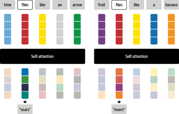
The end result is that the token ‘flies’ will receive the context of ‘soars’ in one sentence and the context of ‘insect’ in the other sentence.

Dimensioning the Attention Mechanism

Other attention mechanisms

There are multiple more advanced attention mechanisms that try in addition to solve the scalability issues from having to manage a \(T \times T\) matrix of attention weights.