You Only Look Once (YOLO)
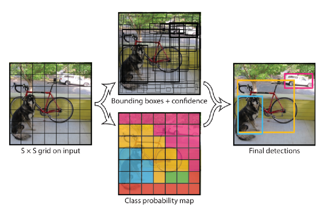
As shown in Figure 1, YOLOv1 partitions the input image into an \(S\times S\) grid. If the center of an object falls in cell \(i\), that cell is responsible for predicting it. Each grid cell outputs \(B\) bounding-box hypotheses and one set of class probabilities over \(C\) classes, yielding an \(S\times S\times (B\cdot 5 + C)\) tensor. For VOC, \(S{=}7\), \(B{=}2\), \(C{=}20\Rightarrow 7\times7\times 30\).
Each bounding box prediction carries five numbers
\[ (x, y, w, h, \text{confidence}), \]
where \((x,y)\) are the box-center offsets relative to the owning cell, and \((w,h)\) are normalized by image width/height. The confidence is intended to equal the IoU between the predicted box and the closest ground-truth box (and be \(0\) when no object is present).
Class-specific confidence at test time
At inference we combine per-cell conditional class probabilities with the per-box confidence to score each box for each class:
\[ \Pr(\text{Class}_i \mid \text{Object}) \cdot \Pr(\text{Object})\cdot \text{IoU}_{\text{pred}}^{\text{truth}} \;=\; \Pr(\text{Class}_i)\cdot \text{IoU}_{\text{pred}}^{\text{truth}}. \tag{1} \]
This produces class-specific confidence scores used before NMS.
Network architecture and activations
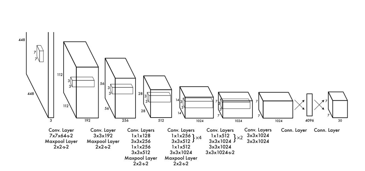
As shown in Figure 2, the detector is a single CNN: 24 conv layers + 2 fully-connected layers; early layers extract features, FC layers map to the \(S\times S\times (B\cdot5+C)\) output. A fast variant reduces conv depth.
Final layer uses a linear activation; all others use leaky ReLU
\[ \phi(x)= \begin{cases} x, & x>0,\\ 0.1x, & \text{otherwise.} \end{cases} \tag{2} \]
Coordinates are normalized as described above.
Training targets and responsibility
Because each cell predicts \(B\) boxes, YOLO assigns “responsibility” to exactly one of the \(B\) predictors for a given object: the predictor whose current box has the highest IoU with that object’s ground-truth. This specialization improves recall.
Consequence for targets:
- Only the responsible predictor for a cell/object receives coordinate and objectness regression targets for that object.
- The other predictor(s) in that cell are trained toward “no object” for confidence, reducing spurious positives.
That assignment happen per-iteration using the model’s current boxes.
The multi-part loss
YOLOv1 optimizes a sum-squared error over location, size, objectness (confidence), and classification, with two balancing coefficients \(\lambda_{\text{coord}}\) and \(\lambda_{\text{noobj}}\). To de-emphasize scale sensitivity, the loss regresses \(\sqrt{w},\sqrt{h}\) instead of \(w,h\).
\[ \begin{aligned} \mathcal{L} = \;& \lambda_{\text{coord}} \sum_{i=1}^{S^2} \sum_{j=1}^{B} \mathbf{1}^{\text{obj}}_{ij} \Big[(x_i-\hat{x}_i)^2 + (y_i-\hat{y}_i)^2\Big] \\ &+ \lambda_{\text{coord}} \sum_{i=1}^{S^2} \sum_{j=1}^{B} \mathbf{1}^{\text{obj}}_{ij} \Big[\big(\sqrt{w_i}-\sqrt{\hat{w}_i}\big)^2 + \big(\sqrt{h_i}-\sqrt{\hat{h}_i}\big)^2\Big] \\ &+ \sum_{i=1}^{S^2}\sum_{j=1}^{B} \mathbf{1}^{\text{obj}}_{ij}\big(C_i-\hat{C}_i\big)^2 + \lambda_{\text{noobj}} \sum_{i=1}^{S^2}\sum_{j=1}^{B} \mathbf{1}^{\text{noobj}}_{ij}\big(C_i-\hat{C}_i\big)^2 \\ &+ \sum_{i=1}^{S^2}\mathbf{1}^{\text{obj}}_{i} \sum_{c\in\mathcal{C}}\big(p_i(c)-\hat{p}_i(c)\big)^2. \end{aligned} \]
Here \(\mathbf{1}^{\text{obj}}_{ij}=1\) iff predictor \(j\) in cell \(i\) is responsible for some object; \(\mathbf{1}^{\text{noobj}}_{ij}=1\) for “no object” cases; \(\lambda_{\text{coord}}{=}5\) and \(\lambda_{\text{noobj}}{=}0.5\). Classification loss is applied only when a cell contains an object.
Optimization details
Typical training recipe (VOC): ~135 epochs, batch size 64, momentum 0.9, weight decay \(5\!\times\!10^{-4}\). LR warmup from \(10^{-3}\) to \(10^{-2}\), then \(10^{-2}\) for 75 epochs, \(10^{-3}\) for 30, \(10^{-4}\) for 30. Regularization via dropout (rate 0.5 after first FC) and data augmentation (random scale/translation up to 20%, exposure/saturation jitters in HSV up to 1.5×).
End-to-end inference
Preprocess: resize the image (e.g., to \(448\times 448\)) and forward once through the CNN.
Decode raw outputs:
- For each cell \(i\) and predictor \(j\): convert normalized \((x,y,w,h)\) to image coordinates; take the predicted confidence \(C_{ij}\).
- Combine with class probabilities \(p_i(c)\) using Eq. (1) to get class-specific scores \(s_{ijc} = p_i(c)\cdot C_{ij}\).
Filter and suppress:
- Discard low-score boxes.
- Perform non-max suppression per class. While not as critical as in proposal-based pipelines, NMS adds ~2–3 mAP points by removing duplicates from neighboring cells.
Strengths and limitations
One-shot, global reasoning; extremely fast.
Different error profile vs. R-CNN family (fewer background false positives, more localization errors).
Limitations: fixed grid capacity (crowded small objects), coarse features due to downsampling, and sensitivity to small-box localization.
Grid cell owns an object if the object’s center falls inside.
Exactly one predictor per owned object learns its geometry (IoU-based responsibility).
Confidence \(=\) objectness \(\times\) IoU; class probs are cell-level. Eq. (1) fuses them into a per-class score.
Loss trades off localization, objectness, and classification with \(\lambda_{\text{coord}},\lambda_{\text{noobj}}\); sizes use square-root to temper scale effects. Eq. (3).