Feature Extraction via Residual Networks
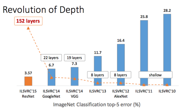
In the figure below we plot the top-5 classification error as a function of depth in CNN architectures. Notice the big jump due to the introduction of the ResNet architecture.

The aim of this section is to provide an alternative view as to why ResNets seem to be able to accommodate much deeper architecture while performing even better that existing architectures for the same depth (e.g. ResNet-18).
The ResNet Architecture

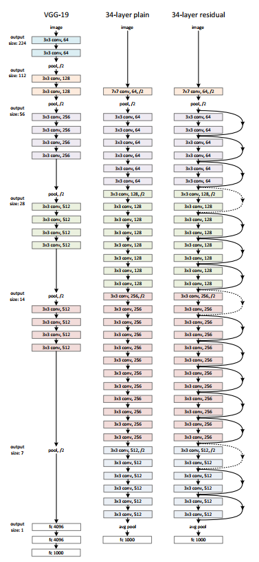
ResNets or residual networks, introduced the concept of the residual. This can be understood looking at a small residual network of three stages. The striking difference between ResNets and earlier architectures are the skip connections. Shortcut connections are those skipping one or more layers. The shortcut connections simply perform identity mapping, and their outputs are added to the outputs of the stacked layers. Identity shortcut connections add neither extra parameter nor computational complexity. The entire network can still be trained end-to-end by SGD with backpropagation, and can be easily implemented using common libraries without modifying the solvers.

Performance advantages of ResNets
Hinton showed that using dropout, dropping out individual neurons during training, leads to a network that is equivalent to averaging over an ensemble of exponentially many networks.We now show that similar ensemble learning performance advantages are present in residual networks.
To do so, we use a simple 3-block network where each layer consists of a residual module \(f_i\) and a skip connection bypassing \(f_i\). Since layers in residual networks can comprise multiple convolutional layers, we refer to them as residual blocks. With \(y_{i-1}\) as is input, the output of the i-th block is recursively defined as
\(y_i = f_i(y_{i−1}) + y_{i−1}\)
where \(f_i(x)\) is some sequence of convolutions, batch normalization, and Rectified Linear Units (ReLU) as nonlinearities. In the figure above we have three blocks. Each \(f_i(x)\) is defined by
\(f_i(x) = W_i^{(1)} * ReLU(B (W_i^{(2)} * RELU(B(x))))\)
where \(W_i^{(1)}\) and \(W_i^{(2)}\) are weight matrices, · denotes convolution, \(B(x)\) is batch normalization and \(RELU(x) ≡ \max(x, 0)\). Other formulations are typically composed of the same operations, but may differ in their order.
This paper analyses the unrolled network and from that analysis we conclude on mainly three advantages of the architecture:
- We see many diverse paths to the gradient as it flows from the \(\hat y\) to the trainable parameter tensors of each layer.
- We see elements of ensemble learning in the formation of the hypothesis \(\hat y\).
- We can eliminate layers from the architecture (blocks) without having to redimension the network, allowing us to trade performance for latancy during inference.
ResNets are commonly used as feature extractors for object detection as in this tutorial.
These networks are a defacto choice today as featurization / backbone networks and they are also extensively used in real time applications.
ResNets and Batch Normalization
This notebook is very instructive of what now is considered a canonical new ResNet block that includes batch normalization.
