Fast RCNN Object Detection
Fast-RCNN is the 2nd generation RCNN that aimed to improve inference time. Apart from the complex training process of RCNN that involved multiple phases across neural and non-neural predictors, its inference involved a forward pass for each of the 2000 proposals through the backbone CNN.
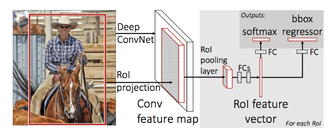
The Fast RCNN architecture is shown below:
Selective search
This is identical to the method we met in RCNN and produces produces region proposals - typically up to 2000 per image.
Modified backbone network
A fully convolutional network network processes the whole image and has several convolutional and max-pooling layers (experiments were done for 5-13 conv and 5 max pooling layers) to produce a feature map.
RoI Pooling Layer
What is an RoI? An RoI is a rectangular window and is mapped (projected) from the proposals produced by selective search (pixel-space) into the feature map. This projection defines for each proposal a four-tuple (x, y, h, w) that specifies its top-left corner (x, y), its height and width (h, w).
The pooling layer uses max pooling to convert the features inside any valid RoI into a small feature map with a fixed spatial extent of H × W (e.g.7 × 7), where H and W are layer hyper-parameters that are independent of any particular RoI.
RoI max pooling works by dividing the h × w RoI window into an H × W grid of sub-windows of approximate size h/H × w/W and then max-pooling the values in each sub-window into the corresponding output grid cell. Pooling is applied independently to each feature map channel, as in standard max pooling.
To accommodate the RoI pooling layer we swap out the last pooling layer of the CNN and endure that the first fully connected layer is dimensionally compatible to accept the RoI pooling layer output.
Bottom line is that for each proposal, a Region of Interest (RoI) pooling layer extracts a fixed-length feature vector from the feature map.
Fully connected classification and regression heads
Each feature vector is fed into a sequence of fully connected (fc) layers that finally branch into two sibling output heads:
- The classification head that produces softmax probability estimates over K object classes plus a catch-all “background” class,
- The Regression head that outputs four (4) real-valued numbers for each of the K object classes. Each set of 4 values encodes refined bounding-box positions for one of the K classes.
Finetuning
The Fast RCNN network is finetuned end-to-end using a multi-task loss function that combines the losses of the classification and bounding-box regression tasks. The loss function is given by:
\[L(\hat y, y, t^y, v) = L_{cls}(\hat y, y) + \lambda[y \geq 1]L_{loc}(t^y, v)\]
where: - \(\hat y\) is the predicted probability of the ground-truth class,
\(y\) is the ground-truth class,
\(t^y\) is the predicted offsets of the predicted bounding-box for class \(y\),
\(v\) is the ground truth bounding-box for class \(y\),
\(L_{cls}\) is the log loss for classification,
\(L_{loc}\) is the smooth L1 loss for bounding-box regression,
\([y \geq 1]\) is an indicator function that is 1 if \(y \geq 1\) and 0 otherwise, and
\(\lambda\) is a hyper-parameter that balances the two loss terms.
\(L_{cls}\) is defined as the usual CE:
\[L_{cls}(\hat y, y) = -\log(\hat y_y)\]
where \(\hat y_y\) is the predicted probability of the ground-truth class.
while \(L_{loc}\) is defined as:
\[L_{loc}(t^y, v) = \sum_{i \in {x, y, w, h}} \mathtt{smooth}_{L1}(t^y_i - v_i)\]
where
\[ \mathtt{smooth}_{L1}(x) = \begin{cases} 0.5 x^2, & \text{if } |x| < 1 \\ |x| - 0.5, & \text{otherwise} \end{cases} \]
Inference
The set of proposals is produced by the same selective search algorithm used in RCNN and its similarly up to 2000 per image.
A Fast RCNN network takes as input an entire image and the set of proposals \(R\). For each proposal the network produces a set of K+1 posterior probabilities and 4K predicted bounding box offsets. We then perform Non-Max Suppression is maintained just like in RCNN to produce the final detection.