Faster RCNN Object Detection
With Faster RCNN, the 3rd generation in the family of region-based detectors, we are replacing the selective search algorithm that is considered computationally expensive, with a neural network called the Region Proposal Network (RPN) that as the name implies produces the proposals. This allows us to call the detector differentiable and therefore train it end-to-end in a much more straightforward way.
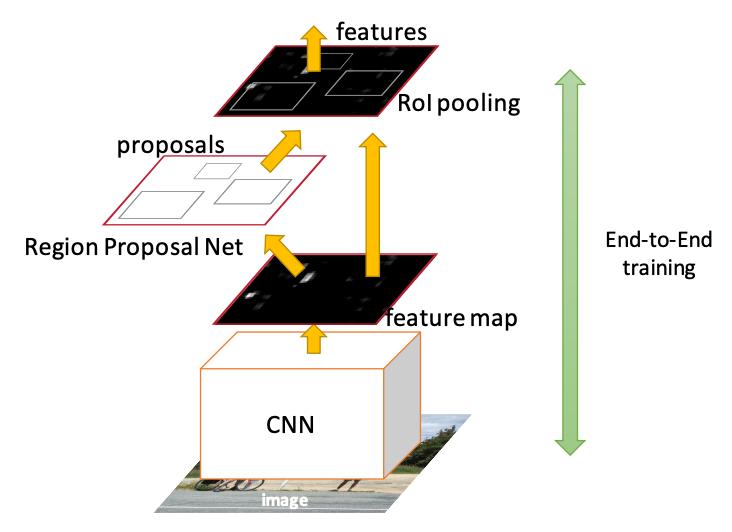
Therefore, in this architecture there is one CNN network that not only produces a global feature map but also produces proposals from the feature map itself rather than the original image, using additional convolutional layers and a sliding window scheme detailed below. Since the RPN component is the key differentiator we limit the discussion to it.
Region Proposal Network (RPN)
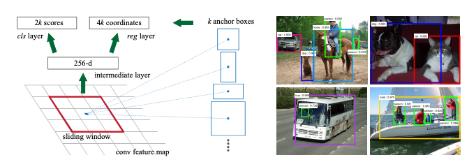
The RPN produces proposals by sliding a window \(n \times n\) over the feature map. At each sliding-window location, we simultaneously predict multiple region proposals, where the number of maximum possible proposals for each location is denoted as \(k\). So the regression layer has \(4k\) outputs encoding the coordinates of \(k\) boxes, and the classification layer outputs \(2k\) scores that represent the probability of the presence of an object or not an object for each proposal.
The \(k\) proposals are parameterized relative to \(k\) reference boxes, which we call anchor boxes. The size can be changed but by default we use 3 scales and 3 aspect ratios, yielding k = 9 anchors at each sliding position. For a feature map of a size \(W × H\) (typically ∼2,400), there are \(W \times H \times k\) anchors in total.
The RPN network produces a classification score i.e. how confident we are that there is an object for each of the anchor boxes as well as the regression on the anchor box coordinates.