Introduction to Recurrent Neural Networks (RNN)
Introduction to Recurrent Neural Networks (RNN)
Sequences
Data streams are everywhere in our lives. Weather station sensor data arrive in streams indexed by time, financial trading data and obviously reading comprehension - one can think of many others. We are interested to fit sequenced data with a model and therefore we need a hypothesis set, that is rich enough for tasks that require some form of memory. In the following we use \(t\) as the index variable without necessarily implying any time semantics.
Dynamical systems are such rich models where the recurrent state evolution can be represented as:
\[\mathbf{s}\_t = f_t(\mathbf{s}\_{t-1}, \mathbf{a}_t ; \mathbf \theta_t)\]
where \(\mathbf s\) is the evolving state, \(\mathbf a\) is an external action or control and \(\mathbf \theta\) is a set of parameters that specify the state evolution model \(f\). This innocent looking equation can capture quite a lot of complexity.
- The state space which is the set of states can depend on \(t\).
- The action space similarly can depend on \(t\)
- Finally, the function that maps previous states and actions to a new state can also depend on \(t\)
So the dynamical system above can indeed offer a very profound modeling flexibility.
RNN Architecture
The RNN architecture is a constrained implementation of the above dynamical system:
\[\mathbf{h}\_t = f(\mathbf{h}\_{t-1}, \mathbf{x}_t ; \mathbf \theta)\]
RNNs implement the same function (parametrized by \(\mathbf \theta\)) across the sequence \(1:\tau\). The state is latent and is denoted with \(\mathbf h\) to match the notation we used earlier for the DNN hidden layers. There is also no dependency on \(t\) of the parameters \(\mathbf \theta\) and this means that the network shares parameters across the sequence. We have seen parameter sharing in CNNs as well but if you recall the sharing was over the relatively small span of the filter. But the most striking difference between CNNs and RNNs is in recursion itself.
 Recursive state representation in RNNs
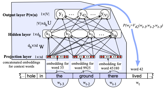
The weights \(\mathbf h\) in CNNs were not a function of previous weights and this means that they cannot remember previous hidden states in the classification or regression task they try to solve. This is perhaps the most distinguishing element of the RNN architecture - its ability to remember via the hidden state who is dimensioned according to the task at hand. There is a way using sliding windows to allow DNNs to remember past inputs as shown in the figure below for an NLP application.
 DNNs can create models from sequential data (such as the language modeling use case shown here). At each step \(t\) the network with a sliding window span of \(\tau=3\) that acts as memory, will concatenate the word embeddings and use a hidden layer \(\mathbf h\) to predict the the next element in the sequence. However, notice that (a) the span is limited and fixed (b) words such as “the ground” will appear in multiple sliding windows forcing the network to learn two different patterns for this constituent (“in the ground”, “the ground there”).
RNNs have a wide variety of architectures.
 From left to right, CNNs, Image Captioning, Sentiment Classification, Machine Translation, Multi-Object Tracking. RNNs are able to work with variable size input and output sequenced data.