Multi-head self-attention
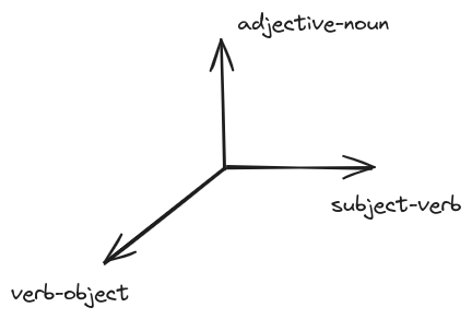
Earlier we have seen examples with the token bear being in multiple grammatical patterns that also influence its meaning. For example, we have seen the subject-verb-object pattern and the subject-verb-adjective-subject pattern. To capture such multiplicities we can use multiple attention heads where each attention head learns a different pattern such as the three shown in figure below.
Think of the multiple heads in transformer architectures to be analogous to the multiple filters we use in CNNs.
if \(H\) is the number of heads, indexed by \(h\), then each head delivers
\[H_h = \mathtt{Attention}(Q_h, K_h, Vh)\]
where \(Q_h, K_h, V_h\) are the query, key and value matrices of the \(h-th\) head.
\[Q_h = X W_h^q\] \[K_h = X W_h^k\] \[V_h = X W_h^v\]
where \(W_h^q, W_h^k, W_h^v\) are the weight matrices of the \(h-th\) head.
The output of the multi-head attention is then given by
\[\hat X = \mathtt{concat}(H_1, H_2, ..., H_H)W^o\]
where \(W^o\) is the output weight matrix with dimensions \(H d_v \times d\) and typically \(d_v = d/H\).
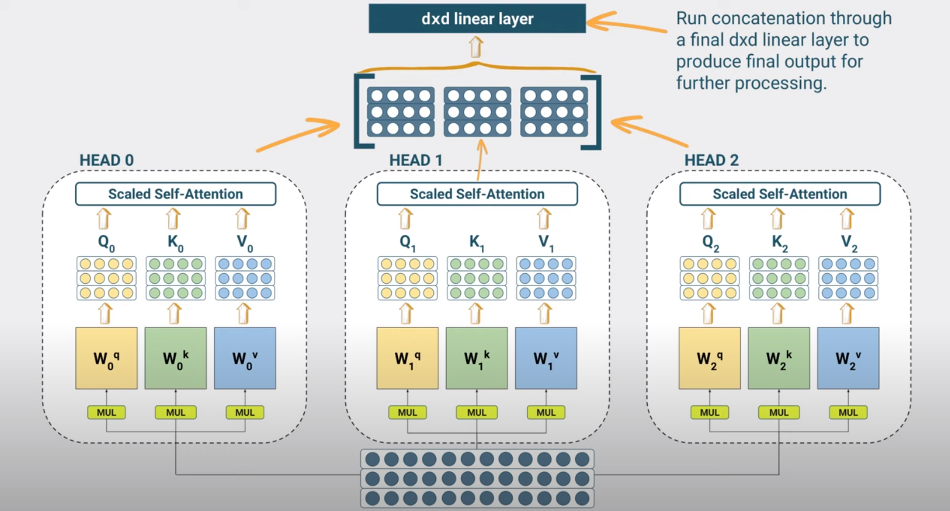
The \(W^o\) matrix and the \(W_h^q, W_h^k, W_h^v\) matrices are learned during training. The complexity of running multiple heads does not scale with the number of heads since as you can also see in the code below we divide the head-size by the number of heads, avoiding a corresponding increase in the number of parameters.
class MultiHeadAttention(nn.Module):
    def __init__(self, config):
        super().__init__()
        embed_dim = config.hidden_size
        num_heads = config.num_attention_heads
        head_dim = embed_dim // num_heads
        self.heads = nn.ModuleList(
            [AttentionHead(embed_dim, head_dim) for _ in range(num_heads)]
        )
        self.output_linear = nn.Linear(embed_dim, embed_dim)

    def forward(self, hidden_state):
        x = torch.cat([h(hidden_state) for h in self.heads], dim=-1)
        x = self.output_linear(x)
        return x
Attention Blocks with Skip Connections
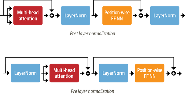
Layer Normalization has been shown to improve training efficiency and therefore we apply layer normalization to the input of the multihead self attention (MHSA).
\[Z = \mathtt{LayerNorm}(\hat X)\]
In addition we borrow the same idea we have seen from ResNet, and add a skip connection from the input to the output of the MHSA.
\[\hat Z = \mathtt{MHSA}(Z) + \hat X\]
We call the above block an attention block and since we know that depth helps in representations learning, we therefore want to stack multiple attention blocks, but before we do so we apply a feedforward layer to the output of each attention block for the reasons we describe below.