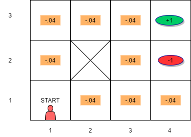
Finding optimal policies in Gridworld
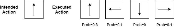
- The environment is stochastic yet fully observable.
- Due to uncertainty, an action causes transition from state to another state with some probability. There is no dependence on previous states.
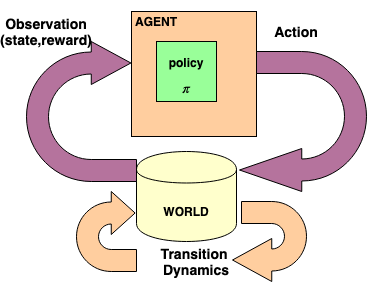
- We now have a sequential decision problem for a fully observable, stochastic environment with Markovian transition model and additive rewards consisting of:
- a set of states \(S\). State at time \(t\) is \(s_t\)
- actions \(A\). Action at time \(t\) is \(a_t\).
- transition model describing outcome of each action in each state \(P( s_{t+1} | s_t,a_t)\)
- reward function \(r_t=R(s_t)\)
MDP Transition Model
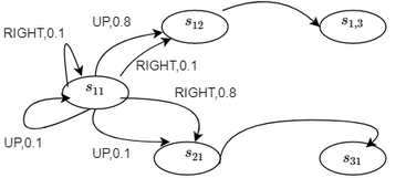
- Transition Model Graph:
- Each node is a state.
- Each edge is the probability of transition
Utility for MDP
- Since we have stochastic environment, we need to take into account the transition probability matrix
- Utility of a state is the immediate reward of the state plus the expected discounted utility of the next state due to the action taken
- Bellman’s Equations: if we choose an action \(a\) then
\(U(s) = R(s) + \gamma \sum_{s^{'}} P(s^{'}| s,a)U(s^{'})\)
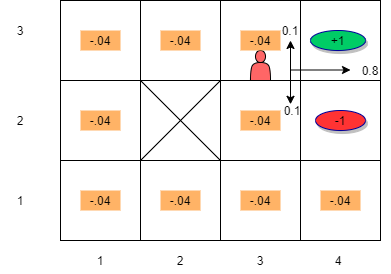
- Suppose robot is in state \(s_{33}\) and the action taken is “RIGHT”. Also assume \(\gamma = 1\)
- We want to compute the utility of this state: \[ U(s_{33}) = R(s_{33}) + \gamma (P(s_{43} | s_{33}, \rightarrow) U(s_{43}) + P(s_{33} | s_{33}, \rightarrow) U(s_{33}) + P(s_{32} | s_{33}, \rightarrow) U(s_{32}))\]
- Substituting we get:
\[U(s_{33}) = R(s_{33}) + \gamma ( (0.8 \times U(s_{43})) + (0.1 \times U(s_{33})) + (0.1 \times U(s_{23})))\]
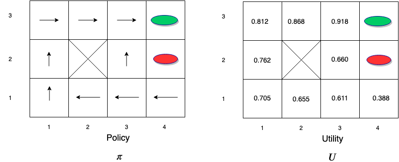
Policy for MDP
If we choose action \(a\) that maximizes future rewards, \(U(s)\) is the maximum we can get over all possible choices of actions and is represented as \(U^{*}(s)\).
We can write this as \[U^*(s) = R(s) + \gamma \underset{a}{ \max} (\sum_{s^{'}} P(s^{'}| s,a)U(s'))\]
The optimal policy (which recommends \(a\) that maximizes U) is given by:
\[\pi^{*}(s) = \underset{a}{\arg \max}(\sum_{s^{'}} P(s^{'}| s,a)U^{*}(s^{'}))\]
Can the above \(2\) be solved directly?
The set of \(|S|\) equations for \(U^*(s)\) cannot be solved directly because they are non-linear due the presence of ‘max’ function.
The set of \(|S|\) equations for \(\pi^*(s)\) cannot be solved directly as it is dependent on unknown \(U^*(s)\).
Optimal Policy for MDP
Value Iteration
- To solve the non-linear equations for \(U^{*}(s)\) we use an iterative approach.
- Steps:
- Initialize estimates for the utilities of states with arbitrary values: \(U(s) \leftarrow 0 \forall s \epsilon S\)
- Next use the iteration step below which is also called Bellman Update:
\[V_{t+1}(s) \leftarrow R(s) + \gamma \underset{a}{ \max} \left[ \sum_{s^{'}} P(s^{'}| s,a) U_t(s^{'}) \right] \forall s \epsilon S\]
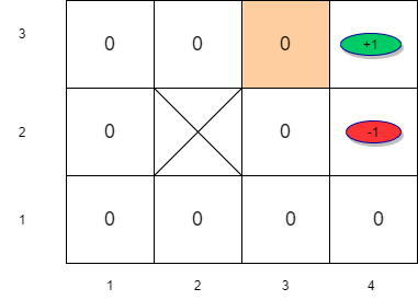
This step is repeated and updated- Let us apply this to the maze example. Assume that \(\gamma = 1\)
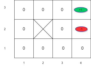 Initialize value estimates to \(0\)
Value Iteration
- Next we want to apply Bellman Update: \[V_{t+1}(s) \leftarrow R(s) + \gamma \max_{a} \left[\sum_{s^\prime} P(s^\prime | s,a)U_t(s^\prime) \right] \forall s \epsilon S\]
- Since we are taking \(\max\) we only need to consider states whose next states have a positive utility value.
- For the remaining states, the utility is equal to the immediate reward in the first iteration.
Value Iteration (t=0)
\[ V_{t+1}(s_{33}) = R(s_{33}) + \gamma \max_a \left[\sum_{s^{'}} P(s^{'}| s_{33},a)U(s^{'}) \right] \forall s \in S \]
\[ V_{t+1}(s_{33}) = -0.04 + \max_a \left[ \sum_{s'} P(s'| s_{33},\uparrow) U_t(s'), \sum_{s'} P(s'| s_{33},\downarrow)U_t(s'), \sum_{s'} P(s'| s_{33},\rightarrow) U_t(s'), \sum_{s'} P(s'| s_{33}, \leftarrow)U_t(s') \right]\]
\[V_{t+1}(s_{33}) = -0.04 + \sum_{s^{'}} P(s^{'}| s_{33},\rightarrow) U_t(s^\prime) \]
\[V_{t+1}(s_{33}) = -0.04 + P(s_{43}|s_{33},\rightarrow)U(s_{43})+P(s_{33}|s_{33},\rightarrow)U(s_{33})+P(s_{32}|s_{33},\rightarrow)U_t(s_{32}) \]
\[V_{t+1}(s_{33}) = -0.04 + 0.8 \times 1 + 0.1 \times 0 + 0.1 \times 0 = 0.76 \]
Value Iteration (t=1)
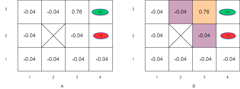 (A) Initial utility estimates for iteration 2. (B) States with next state positive utility
\[V_{t+1}(s_{33}) = -0.04 + P(s_{43}|s_{33},\rightarrow)U_t(s_{43})+P(s_{33}|s_{33},\rightarrow)U_t(s_{33}) +P(s_{32}|s_{33},\rightarrow)U_t(s_{32}) \]
\[V_{t+1}(s_{33}) = -0.04 + 0.8 \times 1 + 0.1 \times 0.76 + 0.1 \times 0 = 0.836\]
\[V_{t+1}(s_{23}) = -0.04 + P(s_{33}|s_{23},\rightarrow)U_t(s_{23})+P(s_{23}|s_{23},\rightarrow)U_t(s_{23}) = -0.04 + 0.8 \times 0.76 = 0.568\]
\[V_{t+1}(s_{32}) = -0.04 + P(s_{33}|s_{32},\uparrow)U_t(s_{33})+P(s_{42}|s_{32},\uparrow)U_t(s_{42}) +P(s_{32}|s_{32},\uparrow)U_t(s_{32})\] \[V_{t+1}(s_{32}) = -0.04 + 0.8 \times 0.76 + 0.1 \times -1 + 0.1 \times 0= 0.468\]
Value Iteration (t=2)
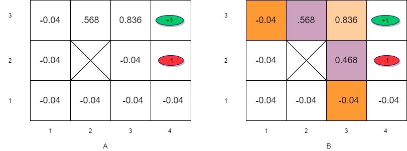 (A)Initial utility estimates for iteration 3. (B) States with next state positive utility
- Information propagates outward from terminal states and eventually all states have correct value estimates
- Notice that \(s_{32}\) has a lower utility compared to \(s_{23}\) due to the red oval state with negative reward next to \(s_{32}\)
Value Iteration - Convergence
- Rate of convergence depends on the maximum reward value and more importantly on the discount factor \(\gamma\).
- The policy that we get from coarse estimates is close to the optimal policy long before \(U\) has converged.
- This means that after a reasonable number of iterations, we could use: \[\pi(s) = \arg \max_a \left[ \sum_{s^{'}} P(s^{'}| s,a)V_{est}(s^{'}) \right]\]
- Note that this is a form of greedy policy.
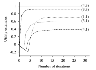 Convergence of utility for the maze problem (Norvig chap 17)
- For the maze problem, convergence is reached within 5 to 10 iterations
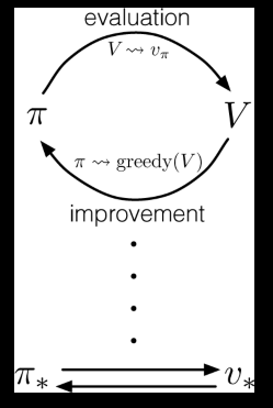
Policy Iteration
Alternates between two steps:
- Policy evaluation: given a policy, find the utility of states
- Policy improvement: given the utility estimates so far, find the best policy
The steps are as follows:
- Compute utility/value of the policy \(U^{\pi}\)
- Update \(\pi\) to be a greedy policy w.r.t. \(U^{\pi}\): \[\pi(s) \leftarrow \arg\max_a \sum_{s^\prime} P(s^\prime|s,a)U^{\pi}(s^\prime)\]
- If the policy changed then return to step \(1\)
Policy improves each step and converges to the optimal policy \(\pi^{*}\)