try:
    from google.colab import output

    print("Running on CoLab")
    #!pip install roboticstoolbox-python>=1.0.2
    !pip install git+https://github.com/petercorke/robotics-toolbox-python@future
    !pip install spatialmath-python>=1.1.5
    !pip install --no-deps rvc3python
    !pip install bdsim
    COLAB = True
except ModuleNotFoundError:
    COLAB = False

from IPython.core.interactiveshell import InteractiveShell

InteractiveShell.ast_node_interactivity = "last_expr_or_assign"
from IPython.display import HTML

%matplotlib inline
import matplotlib.pyplot as plt

# add RTB examples folder to the path
import sys, os.path
import RVC3 as rvc

sys.path.append(os.path.join(rvc.__path__[0], "models"))

# helper function to run bdsim in a subprocess and transfer results using a pickle file
import pickle


def run_shell(tool, **params):
    global out
    pyfile = os.path.join(rvc.__path__[0], "models", tool + ".py")
    cmd = f"python {pyfile} -H +a -o"
    for key, value in params.items():
        cmd += f' --global "{key}={value}"'
    print(cmd)
    os.system(cmd)
    with open("bd.out", "rb") as f:
        out = pickle.load(f)


# ------ standard imports ------ #
import numpy as np
import math
from math import pi

np.set_printoptions(
    linewidth=120,
    formatter={"float": lambda x: f"{0:8.4g}" if abs(x) < 1e-10 else f"{x:8.4g}"},
)
np.random.seed(0)
from spatialmath import *
from spatialmath.base import *
from roboticstoolbox import *Wheeled Robot Models
Robotics, Vision & Control 3e: for Python
Copyright (c) 2021- Peter Corke
4.1 Wheeled Mobile Robots
4.1.1 Car-Like Mobile Robots
NOTE
There are issues in running bdsim from inside Jupyter. We have two options, disable all graphics (which is a bit dull) or run bdsim from a subprocess with its own popout windows.
For Colab we can only do the first option.
Otherwise, we use the wrapper functionrun_shell() defined in the first cell to spawn a new Python instance to run the block diagram which will pop up new windows on your screen to display a simple animation showing the vehicle’s motion in the plane. This makes it a bit harder to get parameters and data between Jupyter and the bdsim simulation, so: * parameter values are passed to bdsim as --global command line options. * the -o command line option to bdsim causes it to write results as a pickle file, which are then imported back into Jupyter.
if COLAB:
    %run -m lanechange -H -g  # no graphics
else:
    run_shell("lanechange")
python /workspaces/rvc3-python/RVC3/models/lanechange.py -H +a -o * Creates Fig 4.5 * Robotics, Vision & Control for Python, P. Corke, Springer 2023. * Copyright (c) 2021- Peter Corke Compiling: ┌────────────┬───────────┬────────┬──────────┬─────────────────────┐ │ block │ type │ inport │ source │ source type │ ├────────────┼───────────┼────────┼──────────┼─────────────────────┤ │ scopexy1.0 │ scopexy1 │ 0 │ vehicle │ ndarray(3,).float64 │ ├────────────┼───────────┼────────┼──────────┼─────────────────────┤ │ speed │ constant │ │ │ │ ├────────────┼───────────┼────────┼──────────┼─���───────────────────┤ │ steering@ │ piecewise │ │ │ │ ├────────────┼───────────┼────────┼──────────┼─────────────────────┤ │ vehicle │ bicycle │ 0 │ speed │ int │ │ │ │ 1 │ steering │ int │ └────────────┴───────────┴────────┴──────────┴─────────────────────┘ Note: @ = event source >>> Start simulation: T = 10, dt = 0.1 Continuous state variables: 3 x0 = [0. 0. 0.] Discrete state variables: 0 Figure(320x320) <<< Simulation complete block diagram evaluations: 730 block diagram exec time: 0.044 ms time steps: 115 integration intervals: 5 simulation results pickled --> bd.out
outt = ndarray:float64 (115,)
x = ndarray:float64 (115, 3)
xnames = ['x', 'y', '$\\theta$'] (list)
ynames = [] (list)plt.plot(out.t, out.x); # q vs time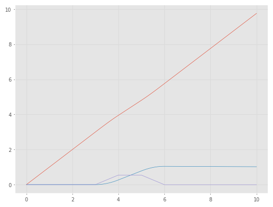
plt.plot(out.x[:, 0], out.x[:, 1]); # x vs y
plt.close(1)4.1.1.1 Driving to a Point
pgoal = (5, 5);qs = (8, 5, pi / 2);if COLAB:
%run -i -m drivepoint -H -g
else:
run_shell("drivepoint", pgoal=pgoal, qs=qs)python /workspaces/rvc3-python/RVC3/models/drivepoint.py -H +a -o --global "pgoal=(5, 5)" --global "qs=(8, 5, 1.5707963267948966)" * Creates Fig 4.7 * Robotics, Vision & Control for Python, P. Corke, Springer 2023. * Copyright (c) 2021- Peter Corke changed value of global pgoal from [5, 5] -> (5, 5) changed value of global qs from [5, 2, 0] -> (8, 5, 1.5707963267948966) WARNING: unused arguments dict_keys(['size', 'shape']) Compiling: ┌───────────────┬─────────────┬────────┬────────────┬─────────────────────┐ │ block │ type │ inport │ source │ source type │ ├───────────────┼─────────────┼────────┼────────────┼─────────────────────┤ │ function.0 │ function │ 0 │ sum.0 │ ndarray(2,).float64 │ ├───────────────┼─────────────┼────────┼────────────┼─────────────────────┤ │ function.1 │ function │ 0 │ sum.0 │ ndarray(2,).float64 │ ├───────────────┼──���──────────┼────────┼────────────┼─────────────────────┤ │ gain.0 │ gain │ 0 │ function.0 │ float │ ├───────────────┼─────────────┼────────┼────────────┼─────────────────────┤ │ gain.1 │ gain │ 0 │ sum.1 │ float │ ├───────────────┼─────────────┼────────┼────────────┼─────────────────────┤ │ goal │ constant │ │ │ │ ├───────────────┼─────────────┼───────��┼────────────┼─────────────────────┤ │ heading │ scope │ 0 │ sum.1 │ float │ ├───────────────┼─────────────┼────────┼────────────┼─────────────────────┤ │ sum.0 │ sum │ 0 │ goal │ ndarray(2,).int64 │ │ │ │ 1 │ xy │ ndarray(2,).float64 │ ├───────────────┼─────────────┼────────┼────────────┼─────────────────────┤ │ sum.1 │ sum │ 0 │ function.1 │ float │ │ │ │ 1 │ theta │ float64 �� ├───────────────┼─────────────┼────────┼────────────┼─────────────────────┤ │ theta │ index │ 0 │ vehicle │ ndarray(3,).float64 │ ├───────────────┼─────────────┼────────┼────────────┼─────────────────────┤ │ vehicle │ bicycle │ 0 │ gain.0 │ float │ │ │ │ 1 │ gain.1 │ float │ ├───────────────┼─────────────┼────────┼────────────┼─────────────────────┤ │ vehicleplot.0 │ vehicleplot │ 0 │ vehicle │ ndarray(3,).float64 │ ├───────────────┼─────────────┼────────┼────────────┼─────────────────────┤ │ velocity │ scope │ 0 │ gain.0 │ float │ ├───────────────┼─────────────┼────────┼────────────┼─────────────────────┤ │ xy │ index │ 0 │ vehicle │ ndarray(3,).float64 │ └───────────────┴─────────────┴────────┴────────────┴─────────────────────┘ >>> Start simulation: T = 10, dt = 0.1 Continuous state variables: 3 x0 = [8. 5. 1.57079633] Discrete state variables: 0 done Figure(320x320) Figure(160x160) Figure(160x160) <<< Simulation complete block diagram evaluations: 614 block diagram exec time: 0.083 ms time steps: 101 integration intervals: 1 simulation results pickled --> bd.out
q = out.x  # configuration vs time
plt.plot(q[:, 0], q[:, 1]);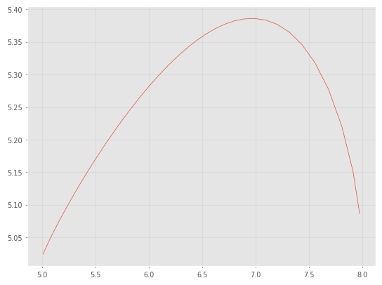
4.1.1.2 Driving Along a Line
L = (1, -2, 4);qs = (8, 5, pi / 2);if COLAB:
%run -m driveline -H -g # no graphics
else:
run_shell("driveline", L=L, qs=qs)python /workspaces/rvc3-python/RVC3/models/driveline.py -H +a -o --global "L=(1, -2, 4)" --global "qs=(8, 5, 1.5707963267948966)" * Creates Fig 4.9 * Robotics, Vision & Control for Python, P. Corke, Springer 2023. * Copyright (c) 2021- Peter Corke changed value of global L from [1, -2, 4] -> (1, -2, 4) changed value of global qs from [8, 5, 1.5707963267948966] -> (8, 5, 1.5707963267948966) WARNING: unused arguments dict_keys(['size', 'shape']) Compiling: ┌───────────────┬─────────────┬────────┬────────────┬─────────────────────┐ │ block │ type │ inport │ source │ source type │ ├───────────────┼─────────────┼────────┼────────────┼─────────────────────┤ │ Kd │ gain │ 0 │ function.0 │ float64 │ ├───────────────┼─────────────┼────────┼────────────┼─────────────────────┤ │ Kh │ gain │ 0 │ sum.0 │ float │ ├───────────────┼──���──────────┼────────┼────────────┼─────────────────────┤ │ constant.0 │ constant │ │ │ │ ├───────────────┼─────────────┼────────┼────────────┼─────────────────────┤ │ constant.1 │ constant │ │ │ │ ├───────────────┼─────────────┼────────┼────────────┼─────────────────────┤ │ function.0 │ function │ 0 │ xy │ ndarray(2,).float64 │ ├───────────────┼─────────────┼───────��┼────────────┼─────────────────────┤ │ heading │ scope │ 0 │ theta │ float64 │ ├───────────────┼─────────────┼────────┼────────────┼─────────────────────┤ │ sum.0 │ sum │ 0 │ constant.1 │ float │ │ │ │ 1 │ theta │ float64 │ ├───────────────┼─────────────┼────────┼────────────┼─────────────────────┤ │ sum.1 │ sum │ 0 │ Kh │ float │ │ │ │ 1 │ Kd │ float64 �� ├───────────────┼─────────────┼────────┼────────────┼─────────────────────┤ │ theta │ index │ 0 │ vehicle │ ndarray(3,).float64 │ ├───────────────┼─────────────┼────────┼────────────┼─────────────────────┤ │ vehicle │ bicycle │ 0 │ constant.0 │ float │ │ │ │ 1 │ sum.1 │ float64 │ ├───────────────┼─────────────┼────────┼────────────┼─────────────────────┤ │ vehicleplot.0 │ vehicleplot │ 0 │ vehicle │ ndarray(3,).float64 │ ├───────────────┼─────────────┼────────┼────────────┼─────────────────────┤ │ xy │ index │ 0 │ vehicle │ ndarray(3,).float64 │ └───────────────┴─────────────┴────────┴────────────┴─────────────────────┘ >>> Start simulation: T = 20, dt = 0.2 Continuous state variables: 3 x0 = [8. 5. 1.57079633] Discrete state variables: 0 done Figure(320x320) Figure(160x160) <<< Simulation complete block diagram evaluations: 608 block diagram exec time: 0.084 ms time steps: 101 integration intervals: 1 simulation results pickled --> bd.out
4.1.1.3 Driving Along a Path
if COLAB:
    %run -m drivepursuit -H -g  # no graphics
else:
    run_shell("drivepursuit")
python /workspaces/rvc3-python/RVC3/models/drivepursuit.py -H +a -o (1925, 2) * Creates Fig 4.11 * Robotics, Vision & Control for Python, P. Corke, Springer 2023. * Copyright (c) 2021- Peter Corke WARNING: unused arguments dict_keys(['size', 'shape']) Compiling: ┌───────────────┬─────────────┬────────┬──────────────┬─────────────────────┐ │ block │ type │ inport │ source │ source type │ ├───────────────┼─────────────┼────────┼──────────────┼─────────────────────┤ │ Kh │ gain │ 0 │ herr │ float │ ├───────────────┼─────────────┼────────┼──────────────┼─────────────────────┤ │ bicycle.0 │ bicycle │ 0 │ speed │ int │ │ │ │ 1 │ Kh │ float │ ├───────────────┼─────────────┼────────┼──────────────┼─────────────────────┤ │ close_enough │ stop │ 0 │ xy │ ndarray(2,).float64 │ ├───────────────┼─────────────┼────────┼──────────────┼─────────────────────┤ │ err │ sum │ 0 │ pure_pursuit │ ndarray(2,).float64 │ │ │ │ 1 │ xy │ ndarray(2,).float64 │ ├───────────────┼─────────────┼────────┼──────────────┼─────────────────────┤ │ h2goal │ function │ 0 │ err │ ndarray(2,).float64 │ ├───────────────┼─────────────┼────────┼──────────────┼─────────────────────┤ │ heading angle │ scope │ 0 │ theta │ float64 │ ├───────────────┼─────────────┼────────┼──────────────┼─────────────────────┤ │ herr │ sum │ 0 │ h2goal │ float │ │ │ │ 1 │ theta │ float64 │ ├───────────────┼─────────────┼────────┼───────────���──┼─────────────────────┤ │ pure_pursuit │ function │ 0 │ xy │ ndarray(2,).float64 │ ├───────────────┼─────────────┼────────┼──────────────┼─────────────────────┤ │ speed │ constant │ │ │ │ ├───────────────┼─────────────┼────────┼──────────────┼─────────────────────┤ │ steer angle │ scope │ 0 │ Kh │ float │ ├───────────────┼─────────────┼────────┼──────────────┼───────��─────────────┤ │ theta │ index │ 0 │ bicycle.0 │ ndarray(3,).float64 │ ├───────────────┼─────────────┼────────┼──────────────┼─────────────────────┤ │ vehicleplot.0 │ vehicleplot │ 0 │ bicycle.0 │ ndarray(3,).float64 │ ├───────────────┼─────────────┼────────┼──────────────┼─────────────────────┤ │ xy │ index │ 0 │ bicycle.0 │ ndarray(3,).float64 │ └───────────────┴─────────────┴────────┴──────────────┴─────────────────────┘ >>> Start simulation: T = 197.5, dt = 1.975 Continuous state variables: 3 x0 = [2. 2. 0.] Discrete state variables: 0 done Figure(320x320) Figure(160x160) Figure(160x160) <<< Simulation complete block diagram evaluations: 680 block diagram exec time: 0.139 ms time steps: 109 integration intervals: 1 simulation results pickled --> bd.out
4.1.1.4 Driving to a Configuration
qg = (5, 5, pi / 2);qs = (9, 5, 0);if COLAB:
%run -m driveconfig -H -g # no graphics
else:
run_shell("driveconfig", qg=qg, qs=qs)python /workspaces/rvc3-python/RVC3/models/driveconfig.py -H +a -o --global "qg=(5, 5, 1.5707963267948966)" --global "qs=(9, 5, 0)" * Creates Fig 4.14 * Robotics, Vision & Control for Python, P. Corke, Springer 2023. * Copyright (c) 2021- Peter Corke WARNING: unused arguments dict_keys(['vlim', 'slim']) WARNING: unused arguments dict_keys(['size', 'shape']) Compiling: alpha -1.5707963267948966 set direction to 1 ┌───────────────┬─────────────┬────────┬──────────────┬─────────────────────┐ │ block │ type │ inport │ source │ source type │ ├───────────────┼─────────────┼────────┼──────────────┼─────────────────────┤ │ Kalpha │ gain │ 0 │ polar[2] │ float64 │ ├───────────────┼─────────────┼────────┼──────────────┼─────────────────────┤ │ Kbeta │ gain │ 0 │ sum.1 │ float │ ├──────────���────┼─────────────┼────────┼──────────────┼─────────────────────┤ │ Krho │ gain │ 0 │ polar[1] │ float │ ├───────────────┼─────────────┼────────┼──────────────┼─────────────────────┤ │ abs │ function │ 0 │ vprod │ float │ ├───────────────┼─────────────┼────────┼──────────────┼─────────────────────┤ │ alpha │ scope │ 0 │ polar[2] │ float64 │ ├───────────────┼─────��───────┼────────┼──────────────┼─────────────────────┤ │ aprod │ prod │ 0 │ sum.2 │ float64 │ │ │ │ 1 │ polar[0] │ int │ │ │ │ 2 │ abs │ float │ ├───────────────┼─────────────┼────────┼──────────────┼─────────────────────┤ │ atan │ function │ 0 │ aprod │ float64 │ ├───────────────┼─────────────┼────────┼──────────────┼─────────────────────┤ │ beta │ scope │ 0 │ sum.1 │ float │ ├───────────────┼─────────────┼────────┼──────────────┼─────────────────────┤ │ close enough │ stop │ 0 │ polar[1] │ float │ ├───────────────┼─────────────┼────────┼──────────────┼─────────────────────┤ │ goal_heading │ constant │ │ │ │ ├───────────────┼─────────────┼────────┼──────────────┼─────────────────────┤ │ goal_pos │ constant │ ��� │ │ ├───────────────┼─────────────┼────────┼──────────────┼─────────────────────┤ │ polar │ function │ 0 │ sum.0 │ ndarray(3,).float64 │ ├───────────────┼─────────────┼────────┼──────────────┼─────────────────────┤ │ sum.0 │ sum │ 0 │ vehicle │ ndarray(3,).float64 │ │ │ │ 1 │ goal_pos │ ndarray(3,).int64 │ ├───────────────┼─────────────┼────────┼──────────────┼─────────────────────┤ │ sum.1 │ sum │ 0 │ polar[3] │ float │ │ │ │ 1 │ goal_heading │ float │ ├───────────────┼─────────────┼────────┼──────────────┼─────────────────────┤ │ sum.2 │ sum │ 0 │ Kalpha │ float64 │ │ │ │ 1 │ Kbeta │ float │ ├───────────────┼─────────────┼────────┼──────────────┼─────────────────────┤ │ vehicle │ bicycle │ 0 │ vprod │ float │ │ │ │ 1 │ atan │ float │ ├───────────────┼─────────────┼────────┼──────────────┼─────────────────────┤ │ vehicleplot.0 │ vehicleplot │ 0 │ vehicle │ ndarray(3,).float64 │ ├───────────────┼─────────────┼────────┼──────────────┼─────────────────────┤ │ vprod │ prod │ 0 │ polar[0] │ int │ │ │ │ 1 │ Krho │ float │ └───────────────┴─────────────┴────────┴──────────────┴─────────────────────┘ >>> Start simulation: T = 10, dt = 0.1 Continuous state variables: 3 x0 = [5. 9. 0.] Discrete state variables: 0 clearing user data done Figure(320x320) Figure(160x160) Figure(160x160) alpha -1.5707963267948966 set direction to 1 --- stop requested at t=7.5111 by close enough <<< Simulation complete block diagram evaluations: 470 block diagram exec time: 0.087 ms time steps: 78 integration intervals: 1 simulation results pickled --> bd.out
q = out.x  # configuration vs time
plt.plot(q[:, 0], q[:, 1]);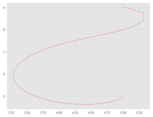
4.2 Aerial Robots
if COLAB:
    %run -m quadrotor -H -g  # no graphics
else:
    run_shell("quadrotor")
python /workspaces/rvc3-python/RVC3/models/quadrotor.py -H +a -o * Creates Fig 4.24 * Robotics, Vision & Control for Python, P. Corke, Springer 2023. * Copyright (c) 2021- Peter Corke Compiling: ┌───────────────────────┬─────────────────┬────────┬────────────────────┬─────────────────────┐ │ block │ type │ inport │ source │ source type │ ├───────────────────────┼─────────────────┼────────┼────────────────────┼─────────────────────┤ │ absval │ function │ 0 │ mixer │ ndarray(4,).float64 │ ├───────────────────────┼─────────────────┼────────┼──────────────────��─┼─────────────────────┤ │ attitude │ scope │ 0 │ slice1.1 │ ndarray(3,).float64 │ ├───────────────────────┼─────────────────┼────────┼────────────────────┼─────────────────────┤ │ attitudecontrol │ function │ 0 │ velcontrol │ ndarray(2,).float64 │ │ │ │ 1 │ quadrotor │ dict │ ├───────────────────────┼─────────────────┼────────┼────────────────────┼─────────────────────┤ │ height demand │ interpolate │ │ │ │ ├───────────────────────┼─────────────────┼────────┼────────────────────┼─────────────────────┤ │ mixer │ multirotormixer │ 0 │ attitudecontrol[0] │ float64 │ │ │ │ 1 │ attitudecontrol[1] │ float64 │ │ │ │ 2 │ yawcontrol │ float64 │ │ │ │ 3 │ zcontrol │ float64 │ ├───────────────────────┼─────────────────┼────────┼────────────────────┼─────────────────────┤ │ multirotorplot.0 │ quadrotorplot │ 0 │ quadrotor │ dict │ ├───────────────────────┼─────────────────┼────────┼────────────────────┼─────────────────────┤ │ position │ scope │ 0 │ slice1.0 │ ndarray(3,).float64 │ ├───────────────────────┼─────────────────┼────────┼────────────────────┼─────────────────────┤ │ quadrotor │ multirotor │ 0 │ mixer │ ndarray(4,).float64 │ ├──────���────────────────┼─────────────────┼────────┼────────────────────┼─────────────────────┤ │ rotor speed (abs.val) │ scope │ 0 │ absval │ ndarray(4,).float64 │ ├───────────────────────┼─────────────────┼────────┼────────────────────┼─────────────────────┤ │ slice1.0 │ slice1 │ 0 │ state │ ndarray(6,).float64 │ ├───────────────────────┼─────────────────┼────────┼────────────────────┼─────────────────────┤ │ slice1.1 │ slice1 │ 0 │ state │ ndarray(6,).float64 │ ├───────────────────────┼─────────────────┼────────┼────────────────────┼─────────────────────┤ │ state │ item │ 0 │ quadrotor │ dict │ ├───────────────────────┼─────────────────┼────────┼────────────────────┼─────────────────────┤ │ velcontrol │ function │ 0 │ xy_demand │ ndarray(2,).float64 │ │ │ │ 1 │ quadrotor │ dict │ ├───────────────────────┼─────────────────┼────────┼────────────────────┼─────────────────────┤ │ waveform.0@ │ waveform │ │ │ │ ├───────────────────────┼─────────────────┼────────┼────────────────────┼─────────────────────┤ │ waveform.1@ │ waveform │ │ │ │ ├───────────────────────┼─────────────────┼────────┼────────────────────┼─────────────────────┤ │ xy_demand │ mux │ 0 │ waveform.0 │ float │ │ │ │ 1 │ waveform.1 │ float │ ├───────────────────────┼─────────────────┼────────┼────────────────────┼─────────────────────┤ │ yaw demand@ │ ramp │ │ │ │ ├───────────────────────┼─────────────────┼────────┼────────────────────┼─────────────��───────┤ │ yawcontrol │ function │ 0 │ yaw demand │ int │ │ │ │ 1 │ quadrotor │ dict │ ├───────────────────────┼─────────────────┼────────┼────────────────────┼─────────────────────┤ │ zcontrol │ function │ 0 │ height demand │ ndarray().float64 │ │ │ │ 1 │ quadrotor │ dict │ └───────────────────────┴─────────────────┴────────┴────────────────────┴────────────���────────┘ Note: @ = event source >>> Start simulation: T = 10, dt = 0.05 Continuous state variables: 12 x0 = [0. 0. 0. 0. 0. 0. 0. 0. 0. 0. 0. 0.] Discrete state variables: 0 Figure(320x320) Figure(160x160) Figure(160x160) Figure(160x160) <<< Simulation complete block diagram evaluations: 1294 block diagram exec time: 0.549 ms time steps: 213 integration intervals: 2 simulation results pickled --> bd.out
t = out.t
x = out.x
x.shape
(213, 12)plt.plot(t, x[:, 0], t, x[:, 1]);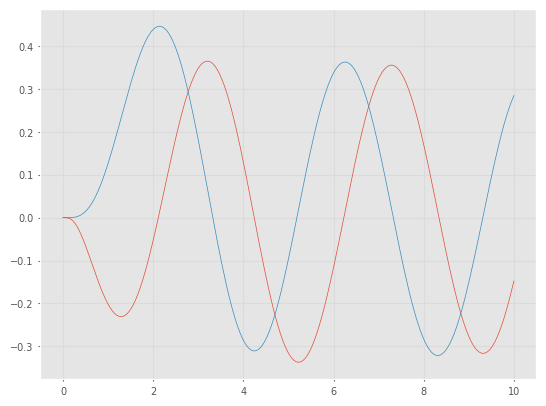
4.4 Wrapping Up
4.4.1 Further Reading
veh = Bicycle(speed_max=1, steer_max=np.deg2rad(30))
veh.q
array([ 0, 0, 0])veh.step([0.3, 0.2])
veh.qarray([ 0.03, 0, 0.006081])veh.deriv(veh.q, [0.3, 0.2])array([ 0.3, 0.001824, 0.06081])