Motion Representations Notebook

Robotics, Vision & Control 3e: for Python

Copyright (c) 2021- Peter Corke

There are some minor code changes compared to the book. These are to support the Matplotlib widget (ipympl) backend. This allows 3D plots to be rotated so the changes are worthwhile.

2.1 Foundations

2.2 Working in Two Dimensions (2D)

2.2.1 Orientation in Two Dimensions

2.2.1.1 2D Rotation Matrix

R = rot2(0.3)

array([[  0.9553,  -0.2955],
       [  0.2955,   0.9553]])

plotvol2(new=True)  # for matplotlib/widget
trplot2(R);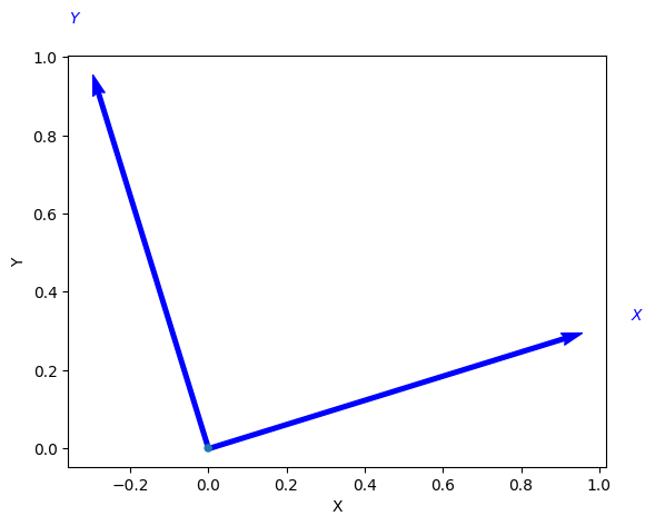

np.linalg.det(R)

0.9999999999999999

np.linalg.det(R @ R)

0.9999999999999998

from sympy import Symbol, Matrix, simplify, pprint

theta = Symbol("theta")
R = Matrix(rot2(theta))  # convert to SymPy matrix

\(\displaystyle \left[\begin{matrix}\cos{\left(\theta \right)} & - \sin{\left(\theta \right)}\\\sin{\left(\theta \right)} & \cos{\left(\theta \right)}\end{matrix}\right]\)

simplify(R * R)

\(\displaystyle \left[\begin{matrix}\cos{\left(2 \theta \right)} & - \sin{\left(2 \theta \right)}\\\sin{\left(2 \theta \right)} & \cos{\left(2 \theta \right)}\end{matrix}\right]\)

R.det()

\(\displaystyle \sin^{2}{\left(\theta \right)} + \cos^{2}{\left(\theta \right)}\)

R.det().simplify()

\(\displaystyle 1\)

2.2.1.2 Matrix Exponential for Rotation

R = rot2(0.3);

L = linalg.logm(R)  # using linalg package of SciPy

array([[       0,     -0.3],
       [     0.3,        0]])

S = vex(L)

array([     0.3])

X = skew(2)

array([[       0,       -2],
       [       2,        0]])

vex(X)

array([       2])

linalg.expm(L)

array([[  0.9553,  -0.2955],
       [  0.2955,   0.9553]])

linalg.expm(skew(S))

array([[  0.9553,  -0.2955],
       [  0.2955,   0.9553]])

2.2.2 Pose in Two Dimensions

2.2.2.1 2D Homogeneous Transformation Matrix

rot2(0.3)

array([[  0.9553,  -0.2955],
       [  0.2955,   0.9553]])

trot2(0.3)

array([[  0.9553,  -0.2955,        0],
       [  0.2955,   0.9553,        0],
       [       0,        0,        1]])

TA = transl2(1, 2) @ trot2(30, "deg")

array([[   0.866,     -0.5,        1],
       [     0.5,    0.866,        2],
       [       0,        0,        1]])

plotvol2([0, 5], new=True)  # new plot with both axes from 0 to 5
trplot2(TA, frame="A", color="b")
T0 = transl2(0, 0)
trplot2(T0, frame="0", color="k")  # reference frame
TB = transl2(2, 1)
trplot2(TB, frame="B", color="r")
TAB = TA @ TB
trplot2(TAB, frame="AB", color="g")
TBA = TB @ TA
trplot2(TBA, frame="BA", color="c")
P = np.array([3, 2])
plot_point(P, "ko", label="P");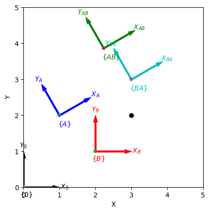

print(TA)
print(P)
np.linalg.inv(TA) @ np.hstack([P, 1])

[[   0.866     -0.5        1]
 [     0.5    0.866        2]
 [       0        0        1]]
[3 2]

array([   1.732,       -1,        1])

h2e(np.linalg.inv(TA) @ e2h(P))

array([[   1.732],
       [      -1]])

homtrans(np.linalg.inv(TA), P)

array([[   1.732],
       [      -1]])

2.2.2.2 Rotating a Coordinate Frame

plotvol2([-5, 4, -1, 5], new=True)  # for matplotlib/widget
T0 = transl2(0, 0)
trplot2(T0, frame="0", color="k")
TX = transl2(2, 3)
trplot2(TX, frame="X", color="b")
TR = trot2(2)
trplot2(TR @ TX, framelabel="RX", color="g")
trplot2(TX @ TR, framelabel="XR", color="g")
C = np.array([3, 2])
plot_point(C, "ko", text="C")
TC = transl2(C) @ TR @ transl2(-C)
trplot2(TC @ TX, framelabel="XC", color="r");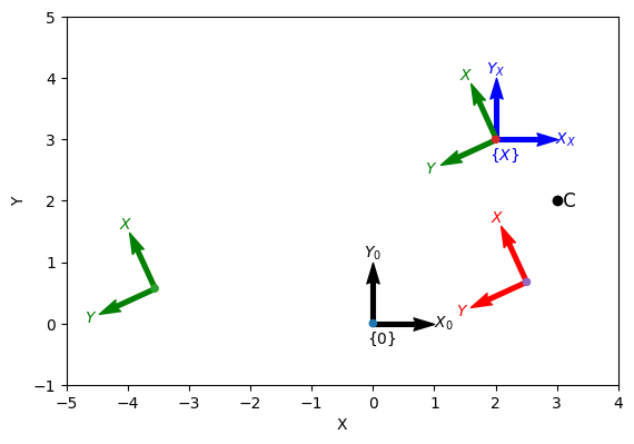

2.2.2.3 Matrix exponential for Pose

L = linalg.logm(TC)

array([[       0,       -2,        4],
       [       2,        0,       -6],
       [       0,        0,        0]])

S = vexa(L)

array([       4,       -6,        2])

linalg.expm(skewa(S))

array([[ -0.4161,  -0.9093,    6.067],
       [  0.9093,  -0.4161,   0.1044],
       [       0,        0,        1]])

X = skewa([1, 2, 3])

array([[       0,       -3,        1],
       [       3,        0,        2],
       [       0,        0,        0]])

vexa(X)

array([       1,        2,        3])

2.2.2.4 2D Twists

S = Twist2.UnitRevolute(C)

(2 -3; 1)

linalg.expm(skewa(2 * S.S))

array([[ -0.4161,  -0.9093,    6.067],
       [  0.9093,  -0.4161,   0.1044],
       [       0,        0,        1]])

S.exp(2)

  -0.4161   -0.9093    6.067     
   0.9093   -0.4161    0.1044    
   0         0         1         

S.pole

array([       3,        2])

S = Twist2.UnitPrismatic([0, 1])

(0 1; 0)

S.exp(2)

   1         0         0         
   0         1         2         
   0         0         1         

T = transl2(3, 4) @ trot2(0.5)

array([[  0.8776,  -0.4794,        3],
       [  0.4794,   0.8776,        4],
       [       0,        0,        1]])

S = Twist2(T)

(3.9372 3.1663; 0.5)

S.w

0.5

S.pole

array([  -3.166,    3.937])

S.exp(1)

   0.8776   -0.4794    3         
   0.4794    0.8776    4         
   0         0         1         

2.3 Working in Three Dimensions (3D)

2.3.1 Orientation in Three Dimensions

2.3.1.1 3D Rotation Matrix

R = rotx(pi / 2)

array([[       1,        0,        0],
       [       0,        0,       -1],
       [       0,        1,        0]])

plotvol3(new=True)  # for matplotlib/widget
trplot(R);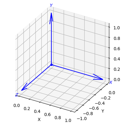

import matplotlib.pyplot as plt
import matplotlib.animation as animation
import numpy as np
from scipy.linalg import logm, expm
import tempfile
import os
from IPython.display import Image, display


def create_rotation_gif(R, filename=None, frames=60, duration=3.0, figsize=(8, 6), dpi=100):
    """
    Create GIF animation of 3D coordinate frame rotation

    Parameters:
    - R: 3x3 rotation matrix
    - filename: output filename (optional, creates temp file if None)
    - frames: number of animation frames
    - duration: animation duration in seconds
    - figsize: figure size tuple
    - dpi: dots per inch for output quality

    Returns:
    - filename of created GIF or IPython Image object
    """
    fig = plt.figure(figsize=figsize, dpi=dpi)
    ax = fig.add_subplot(111, projection="3d")

    # Generate smooth rotation sequence
    angles = np.linspace(0, 1, frames)

    # Create rotation interpolation
    if np.allclose(R, np.eye(3)):
        # If identity matrix, create a full rotation for visualization
        R_seq = [expm(t * 2 * np.pi * np.array([[0, -1, 0], [1, 0, 0], [0, 0, 0]])) for t in angles]
    else:
        # Interpolate to the target rotation
        try:
            log_R = logm(R)
            R_seq = [expm(t * log_R) for t in angles]
        except:
            # Fallback for problematic matrices
            R_seq = [R for _ in angles]

    def animate_frame(frame_idx):
        ax.clear()
        ax.set_xlim([-1.2, 1.2])
        ax.set_ylim([-1.2, 1.2])
        ax.set_zlim([-1.2, 1.2])

        R_current = R_seq[frame_idx]
        origin = [0, 0, 0]

        # Draw reference coordinate frame (fixed, gray)
        ax.quiver(
            *origin,
            1,
            0,
            0,
            color="lightgray",
            arrow_length_ratio=0.1,
            linewidth=1,
            alpha=0.5,
        )
        ax.quiver(
            *origin,
            0,
            1,
            0,
            color="lightgray",
            arrow_length_ratio=0.1,
            linewidth=1,
            alpha=0.5,
        )
        ax.quiver(
            *origin,
            0,
            0,
            1,
            color="lightgray",
            arrow_length_ratio=0.1,
            linewidth=1,
            alpha=0.5,
        )

        # Draw animated coordinate axes with proper colors and labels
        # X-axis (red)
        ax.quiver(
            *origin,
            R_current[0, 0],
            R_current[1, 0],
            R_current[2, 0],
            color="red",
            arrow_length_ratio=0.1,
            linewidth=3,
        )
        ax.text(
            R_current[0, 0] * 1.3,
            R_current[1, 0] * 1.3,
            R_current[2, 0] * 1.3,
            "X",
            color="red",
            fontsize=12,
            fontweight="bold",
        )

        # Y-axis (green)
        ax.quiver(
            *origin,
            R_current[0, 1],
            R_current[1, 1],
            R_current[2, 1],
            color="green",
            arrow_length_ratio=0.1,
            linewidth=3,
        )
        ax.text(
            R_current[0, 1] * 1.3,
            R_current[1, 1] * 1.3,
            R_current[2, 1] * 1.3,
            "Y",
            color="green",
            fontsize=12,
            fontweight="bold",
        )

        # Z-axis (blue)
        ax.quiver(
            *origin,
            R_current[0, 2],
            R_current[1, 2],
            R_current[2, 2],
            color="blue",
            arrow_length_ratio=0.1,
            linewidth=3,
        )
        ax.text(
            R_current[0, 2] * 1.3,
            R_current[1, 2] * 1.3,
            R_current[2, 2] * 1.3,
            "Z",
            color="blue",
            fontsize=12,
            fontweight="bold",
        )

        # Set labels and title
        ax.set_xlabel("X")
        ax.set_ylabel("Y")
        ax.set_zlabel("Z")
        ax.set_title(f"Coordinate Frame Animation\nFrame {frame_idx + 1}/{frames}")

        # Keep camera view fixed for better visualization of rotation
        ax.view_init(elev=20, azim=45)

    # Create animation
    anim = animation.FuncAnimation(
        fig,
        animate_frame,
        frames=frames,
        interval=duration * 1000 / frames,
        repeat=True,
    )

    # Save as GIF using Pillow writer (more reliable than ffmpeg)
    if filename is None:
        with tempfile.NamedTemporaryFile(suffix=".gif", delete=False) as tmp:
            filename = tmp.name

        # Save with Pillow writer
        writer = animation.PillowWriter(fps=frames / duration)
        anim.save(filename, writer=writer)

        plt.close(fig)

        # Read and return as IPython Image for Jupyter display
        with open(filename, "rb") as f:
            gif_data = f.read()

        # Clean up temporary file
        os.unlink(filename)

        return Image(data=gif_data, format="gif")
    else:
        # Save to specified file
        writer = animation.PillowWriter(fps=frames / duration)
        anim.save(filename, writer=writer)
        plt.close(fig)
        return filename


def tranimate_gif(R, save_path=None, **kwargs):
    """
    GIF-based replacement for tranimate function

    Parameters:
    - R: rotation matrix
    - save_path: optional path to save GIF
    - **kwargs: additional animation parameters

    Returns:
    - IPython Image object for Jupyter display or filename if saved
    """
    return create_rotation_gif(R, filename=save_path, **kwargs)

# Replace the problematic cell with:
# ...existing code...
# from spatialmath.base.gif_animate import tranimate_gif

R = rotx(pi / 2)

# Create and display GIF animation instead of HTML5 video
gif_animation = tranimate_gif(R, frames=60, duration=3.0)
display(gif_animation)

# Optional: Save the animation for use in documentation
# tranimate_gif(R, save_path="figures/rotation_x_90deg.gif")

<IPython.core.display.Image object>

Robust, portable animation in Jupyter notebooks is challenging. We’ve replaced the original tranimate HTML5 video animations with a custom GIF-based animation function for better compatibility:

gif_animation = tranimate_gif(R, frames=60, duration=3.0)
display(gif_animation)

If you wish to animate a coordinate frame from a regular Python script, you can still use the simpler syntax:

tranimate(R)

plotvol3(new=True)  # for matplotlib/widget
trplot(R, anaglyph=True)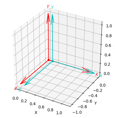

R = rotx(pi / 2) @ roty(pi / 2)
trplot(R);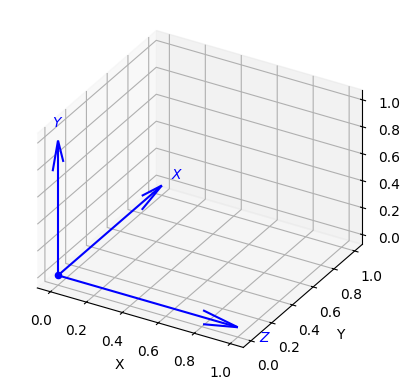

Ryx = roty(pi / 2) @ rotx(pi / 2)

array([[       0,        1,        0],
       [       0,        0,       -1],
       [      -1,        0,        0]])

plotvol3(new=True)  # for matplotlib/widget
trplot(Ryx);

2.3.1.2 Three-Angle Representations

R = rotz(0.1) @ roty(0.2) @ rotz(0.3);

R = eul2r(0.1, 0.2, 0.3)

array([[  0.9021,  -0.3836,   0.1977],
       [  0.3875,   0.9216,  0.01983],
       [ -0.1898,  0.05871,   0.9801]])

gamma = tr2eul(R)

array([     0.1,      0.2,      0.3])

R = eul2r(0.1, -0.2, 0.3)

array([[  0.9021,  -0.3836,  -0.1977],
       [  0.3875,   0.9216, -0.01983],
       [  0.1898, -0.05871,   0.9801]])

gamma = tr2eul(R)

array([  -3.042,      0.2,   -2.842])

eul2r(gamma)

array([[  0.9021,  -0.3836,  -0.1977],
       [  0.3875,   0.9216, -0.01983],
       [  0.1898, -0.05871,   0.9801]])

R = eul2r(0.1, 0, 0.3)

array([[  0.9211,  -0.3894,        0],
       [  0.3894,   0.9211,        0],
       [       0,        0,        1]])

tr2eul(R)

array([       0,        0,      0.4])

R = rpy2r(0.1, 0.2, 0.3, order="zyx")

array([[  0.9363,  -0.2751,   0.2184],
       [  0.2896,   0.9564, -0.03696],
       [ -0.1987,  0.09784,   0.9752]])

gamma = tr2rpy(R, order="zyx")

array([     0.1,      0.2,      0.3])

R = rpy2r(0.1, 0.2, 0.3, order="xyz")

array([[  0.9752, -0.09784,   0.1987],
       [  0.1538,   0.9447,  -0.2896],
       [ -0.1593,    0.313,   0.9363]])

gamma = tr2rpy(R, order="xyz")

array([     0.1,      0.2,      0.3])

The next cell will launch an interactive tool (using the Swift visualizer) in a new browser tab. Close the browser tab when you are done with it.

You might also have to stop the cell from executing, by pressing the stop button for the cell. It may terminate with lots of errors, don’t panic.

if COLAB or not SWIFT:
    print("we can't run this demo from the Colab environment (yet)")
else:
    %run -m tripleangledemo

we can't run this demo from the Colab environment (yet)

2.3.1.3 Singularities and Gimbal Lock

2.3.1.4 Two-Vector Representation

a = [0, 0, -1]

[0, 0, -1]

o = [1, 1, 0]

[1, 1, 0]

R = oa2r(o, a)

array([[ -0.7071,   0.7071,        0],
       [  0.7071,   0.7071,        0],
       [       0,        0,       -1]])

2.3.1.5 Rotation about an Arbitrary Vector

R = rpy2r(0.1, 0.2, 0.3);

theta, v = tr2angvec(R)

theta

0.3655021863566987

v

array([  0.1886,   0.5834,     0.79])

e, x = np.linalg.eig(R)

e

array([0.93394439+0.35741835j, 0.93394439-0.35741835j, 1.        +0.j        ])

x

array([[ 0.69442042+0.j        ,  0.69442042-0.j        ,  0.18857511+0.j        ],
       [-0.07921035-0.56882404j, -0.07921035+0.56882404j,  0.58337798+0.j        ],
       [-0.10726605+0.42004668j, -0.10726605-0.42004668j,  0.79000605+0.j        ]])

theta = np.angle(e[0])

0.3655021863566988

R = angvec2r(0.3, [1, 0, 0])

array([[       1,        0,        0],
       [       0,   0.9553,  -0.2955],
       [       0,   0.2955,   0.9553]])

2.3.1.6 Matrix Exponential for Rotation

R = rotx(0.3)

array([[       1,        0,        0],
       [       0,   0.9553,  -0.2955],
       [       0,   0.2955,   0.9553]])

L = linalg.logm(R)

array([[       0,        0,        0],
       [       0,        0,     -0.3],
       [       0,      0.3,        0]])

S = vex(L)

array([     0.3,        0,        0])

L = trlog(R);

linalg.expm(L)

array([[       1,        0,        0],
       [       0,   0.9553,  -0.2955],
       [       0,   0.2955,   0.9553]])

trexp(L);

linalg.expm(skew(S))

array([[       1,        0,        0],
       [       0,   0.9553,  -0.2955],
       [       0,   0.2955,   0.9553]])

R = rotx(0.3);

R = linalg.expm(0.3 * skew([1, 0, 0]));

X = skew([1, 2, 3])

array([[ 0, -3,  2],
       [ 3,  0, -1],
       [-2,  1,  0]])

vex(X)

array([       1,        2,        3])

2.3.1.7 Unit Quaternions

q = UnitQuaternion(rpy2r(0.1, 0.2, 0.3))

 0.9833 <<  0.0343,  0.1060,  0.1436 >>

q = q * q;

q.inv()

 0.9339 << -0.0674, -0.2085, -0.2824 >>

q * q.inv()

 1.0000 <<  0.0000,  0.0000,  0.0000 >>

q / q

 1.0000 <<  0.0000,  0.0000,  0.0000 >>

q.R

array([[  0.7536,  -0.4993,   0.4275],
       [  0.5555,   0.8315, -0.008145],
       [ -0.3514,   0.2436,    0.904]])

q * [1, 0, 0]

array([  0.7536,   0.5555,  -0.3514])

plotvol3(new=True)  # for matplotlib/widget
q.plot();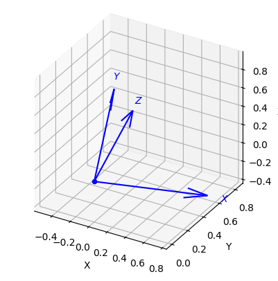

2.3.2 Pose in Three Dimensions

2.3.2.1 Homogeneous Transformation Matrix

T = transl(2, 0, 0) @ trotx(pi / 2) @ transl(0, 1, 0)

array([[       1,        0,        0,        2],
       [       0,        0,       -1,        0],
       [       0,        1,        0,        1],
       [       0,        0,        0,        1]])

plotvol3(new=True)  # for matplotlib/widget
trplot(T);

t2r(T)

array([[       1,        0,        0],
       [       0,        0,       -1],
       [       0,        1,        0]])

transl(T)

array([       2,        0,        1])

2.3.2.2 Matrix exponential for Pose

T = transl(2, 3, 4) @ trotx(0.3)

array([[       1,        0,        0,        2],
       [       0,   0.9553,  -0.2955,        3],
       [       0,   0.2955,   0.9553,        4],
       [       0,        0,        0,        1]])

L = linalg.logm(T)

array([[       0,        0,        0,        2],
       [       0,        0,     -0.3,    3.577],
       [       0,      0.3,        0,     3.52],
       [       0,        0,        0,        0]])

S = vexa(L)

array([       2,    3.577,     3.52,      0.3,        0,        0])

linalg.expm(skewa(S))

array([[       1,        0,        0,        2],
       [       0,   0.9553,  -0.2955,        3],
       [       0,   0.2955,   0.9553,        4],
       [       0,        0,        0,        1]])

X = skewa([1, 2, 3, 4, 5, 6])

array([[       0,       -6,        5,        1],
       [       6,        0,       -4,        2],
       [      -5,        4,        0,        3],
       [       0,        0,        0,        0]])

vexa(X)

array([       1,        2,        3,        4,        5,        6])

2.3.2.3 3D Twists

S = Twist3.UnitRevolute([1, 0, 0], [0, 0, 0])

(0 0 0; 1 0 0)

linalg.expm(0.3 * skewa(S.S));  # different to book, see §2.2.1.2

S.exp(0.3)

   1         0         0         0         
   0         0.9553   -0.2955    0         
   0         0.2955    0.9553    0         
   0         0         0         1         

S = Twist3.UnitRevolute([0, 0, 1], [2, 3, 2], 0.5)

(3 -2 0.5; 0 0 1)

X = transl(3, 4, -4);

for theta in np.arange(0, 15, 0.3):
    trplot(S.exp(theta).A @ X, style="rviz", width=2)

L = S.line()
L.plot("k:", linewidth=2);

Axes3D(0.125,0.11;0.775x0.77)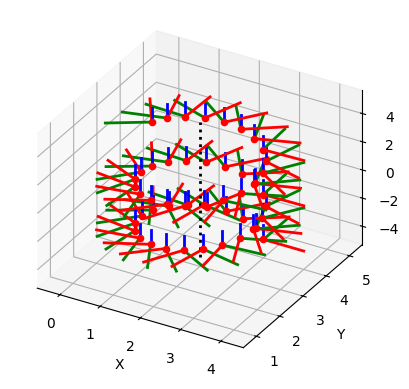

S = Twist3.UnitPrismatic([0, 1, 0])

(0 1 0; 0 0 0)

S.exp(2)

   1         0         0         0         
   0         1         0         2         
   0         0         1         0         
   0         0         0         1         

T = transl(1, 2, 3) @ eul2tr(0.3, 0.4, 0.5)
S = Twist3(T)

(1.1204 1.6446 3.1778; 0.041006 0.4087 0.78907)

S.w

array([ 0.04101,   0.4087,   0.7891])

S.pole

array([0.001138,   0.8473,  -0.4389])

S.pitch

3.2256216289351296

S.theta

0.8895797456112914

2.4 Advanced Topics

2.4.5 Distance Between Orientations

UnitQuaternion.Rx(pi / 2).angdist(UnitQuaternion.Rz(-pi / 2))

1.0471975511965976

2.4.6 Normalization

R = np.eye(3, 3)
np.linalg.det(R) - 1

0.0

for i in range(100):
    R = R @ rpy2r(0.2, 0.3, 0.4)
np.linalg.det(R) - 1

5.773159728050814e-15

R = trnorm(R);

np.linalg.det(R) - 1

2.220446049250313e-16

q = q.unit();

# T = T1 @ T2
# q = q1 @ q2

2.4.8 More About Twists

S = Twist3.UnitRevolute([1, 0, 0], [0, 0, 0])

(0 0 0; 1 0 0)

S.S
S.v
S.w

array([       1,        0,        0])

S.skewa()

array([[       0,        0,        0,        0],
       [       0,        0,       -1,        0],
       [       0,        1,        0,        0],
       [       0,        0,        0,        0]])

trexp(0.3 * S.skewa())

array([[       1,        0,        0,        0],
       [       0,   0.9553,  -0.2955,        0],
       [       0,   0.2955,   0.9553,        0],
       [       0,        0,        0,        1]])

S.exp(0.3)

   1         0         0         0         
   0         0.9553   -0.2955    0         
   0         0.2955    0.9553    0         
   0         0         0         1         

S2 = S * S
S2.printline(orient="angvec", unit="rad")

t = 0, 0, 0; angvec = (2 | 1, 0, 0)

line = S.line()

{ 0 0 0; 1 0 0}

plotvol3([-5, 5], new=True)  # setup volume in which to display the line
line.plot("k:", linewidth=2);

Axes3D(0.125,0.11;0.775x0.77)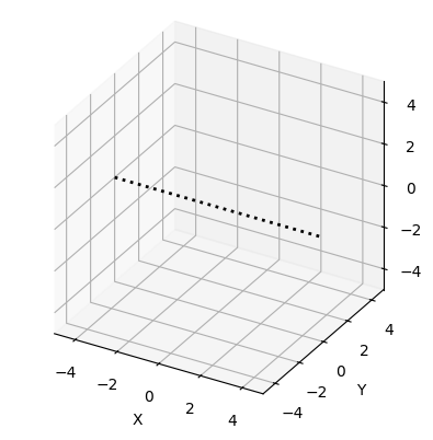

T = transl(1, 2, 3) @ eul2tr(0.3, 0.4, 0.5)
S = Twist3(T)

(1.1204 1.6446 3.1778; 0.041006 0.4087 0.78907)

S / S.theta

(1.2594 1.8488 3.5722; 0.046096 0.45943 0.88702)

S.unit();

S.exp(0)

   1         0         0         0         
   0         1         0         0         
   0         0         1         0         
   0         0         0         1         

S.exp(1)

   0.6305   -0.6812    0.372     1         
   0.6969    0.7079    0.1151    2         
  -0.3417    0.1867    0.9211    3         
   0         0         0         1         

S.exp(0.5)

   0.9029   -0.3796    0.2017    0.5447    
   0.3837    0.9232    0.01982   0.9153    
  -0.1937    0.05949   0.9793    1.542     
   0         0         0         1         

NOTE

The next cell will launch an interactive tool (using the Swift visualizer) in a new browser tab. Close the browser tab when you are done with it.

You might also have to stop the cell from executing, by pressing the stop button for the cell. It may terminate with lots of errors, don’t panic.

if COLAB or not SWIFT:
    print("we can't run this demo from the Colab environment (yet)")
else:
    %run -m twistdemo

we can't run this demo from the Colab environment (yet)

2.5 Using the Toolbox

from spatialmath.base import *

from spatialmath import *

R = rotx(0.3)  # create SO(3) matrix as NumPy array
type(R)
R = SO3.Rx(0.3)  # create SO3 object
type(R)

spatialmath.pose3d.SO3

R.A

array([[       1,        0,        0],
       [       0,   0.9553,  -0.2955],
       [       0,   0.2955,   0.9553]])

R = SO3(rotx(0.3))  # convert an SO(3) matrix
R = SO3.Rz(0.3)  # rotation about z-axis
R = SO3.RPY(10, 20, 30, unit="deg")  # from roll-pitch-yaw angles
R = SO3.AngleAxis(0.3, (1, 0, 0))  # from angle and rotation axis
R = SO3.EulerVec((0.3, 0, 0));  # from an Euler vector

R.rpy()  # convert to roll-pitch-yaw angles
R.eul()  # convert to Euler angles
R.printline();  # compact single-line print

 rpy/zyx = 17.2°, 0°, 0°

R = SO3.RPY(10, 20, 30, unit="deg")  # create an SO(3) rotation
T = SE3.RPY(10, 20, 30, unit="deg")  # create a purely rotational SE(3)
S = Twist3.RPY(10, 20, 30, unit="deg")  # create a purely rotational twist
q = UnitQuaternion.RPY(10, 20, 30, unit="deg");  # create a unit quaternion

TA = SE2(1, 2) * SE2(30, unit="deg")
type(TA)

spatialmath.pose2d.SE2

TA

   0.866    -0.5       1         
   0.5       0.866     2         
   0         0         1         

TA = SE2(1, 2, 30, unit="deg");

TA.R
TA.t

array([       1,        2])

plotvol2(new=True)  # for matplotlib/widget
TA.plot(frame="A", color="b");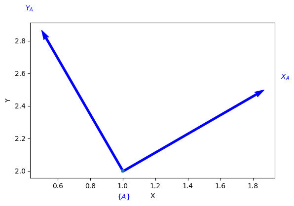

TA.printline()

t = 1, 2; 30°

P = [3, 2]
TA.inv() * P

array([[   1.732],
       [      -1]])

R = SO3.Rx(np.linspace(0, 1, 5))
len(R)
R[3]

   1         0         0         
   0         0.7317   -0.6816    
   0         0.6816    0.7317    

R * [1, 2, 3]

array([[       1,        1,        1,        1,        1],
       [       2,    1.196,   0.3169,  -0.5815,   -1.444],
       [       3,    3.402,    3.592,    3.558,    3.304]])