Configuration Space Topology
A robot is mechanically constructed by connecting a set of bodies, called links,to each other using various types of joints.Actuators, such as electric motors,deliver forces or torques that cause the robot’s links to move. Usually an end-effector, such as a gripper or hand for grasping and manipulating objects, is attached to a specific link.
Although some sections include material that spans many types of robots, in this version of the course we emphasize on robots with egomotion that move in planar surfaces and they have no gripping capability.
Perhaps the most fundamental question one can ask is what is the robot’s configuration. The answe is the specification of the positions of all points of the robot’s mechanisms. As an example, the configuration of the coin shown in Figure 1 lying headsup on a flat table can be described by three coordinates: two coordinates \((x,y)\) that specify the location of a particular point on the coin, and one coordinate (\(θ\)) that specifies the coin’s orientation.
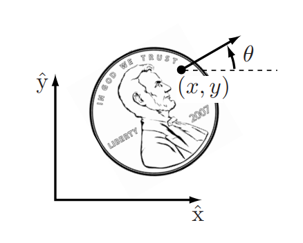
The above coordinates all take values over a continuous range of real numbers. The number of degrees of freedom (dof) of a robot is the smallest number of real-valued coordinates needed to represent its configuration. The coin lying heads up on a table has three degrees of freedom. Even if the coin could lie either heads up or tails up, its configuration space still would have only three degrees of freedom; a fourth variable, representing which side of the coin faces up, takes values in the discrete set {heads,tails}, and not over a continuous range of real values like the other three coordinates.
The n-dimensional space containing all possible configurations of the robot is called the configuration space (C-space). The configuration of a robot is represented by a point in its C-space.
As another example, a plane has 6-DoF, three angles and three cartesian coordinates, as shown in Figure 2.

Constraints and Joints
A robot however cannot actually move everywhere and the feasible motions depend on the configuration of its actuators and the constraints the robot has with the environment. Joints constrain the motion of any rigid body and reduce the overall degrees of freedom. This observation suggests a formula for determining the number of degrees of freedom of a robot, known as Grubler’s rule:
\[ \mathrm{dof} = m \left( N - 1 - J \right) + \sum_{i=1}^{J} f_i \]
where \(m = 3\) for planar mechanisms and \(m = 6\) for spatial mechanisms, \(N\) is the number of links (including the ground link), \(J\) is the number of joints, and \(f_i\) is the number of degrees of freedom of joint \(i\). If the constraints enforced by the joints are not independent, then Grübler’s formula provides a lower bound on the number of degrees of freedom. As an example, as shown in Figure 3, a revolute joint can be viewed as allowing one freedom of motion between two rigid bodies in space, or it can be viewed as providing five constraints on the motion of one rigid body relative to the other.
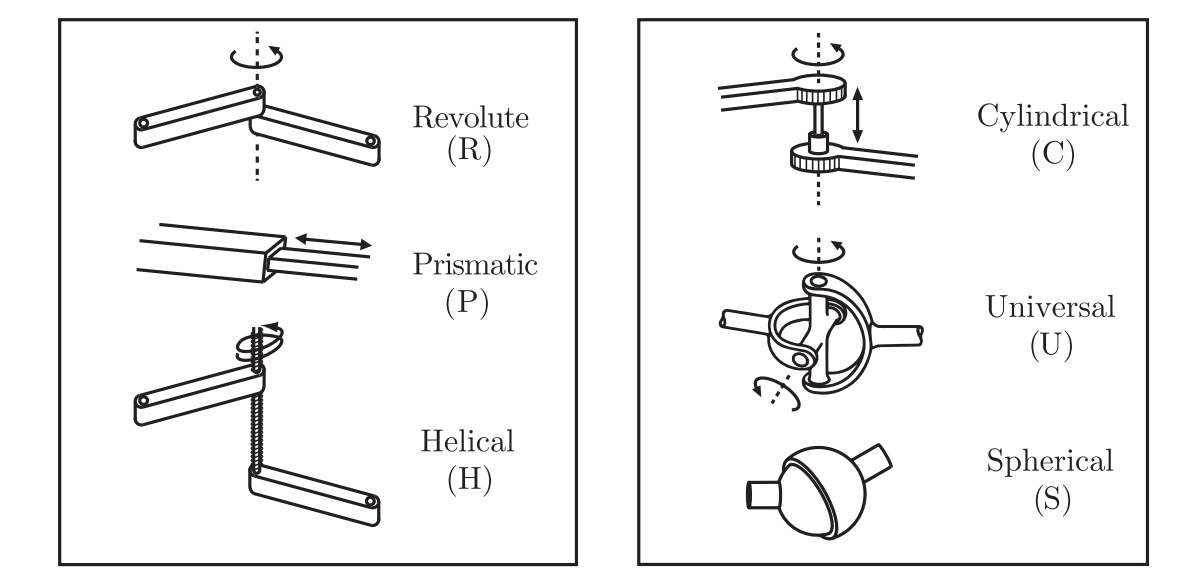
| Joint type | DoF | Constraints between two planar rigid bodies | Constraints between two spatial rigid bodies |
|---|---|---|---|
| Revolute (R) | 1 | 2 | 5 |
| Prismatic (P) | 1 | 2 | 5 |
| Helical (H) | 1 | N/A | 5 |
| Cylindrical (C) | 2 | N/A | 4 |
| Universal (U) | 2 | N/A | 4 |
| Spherical (S) | 3 | N/A | 3 |
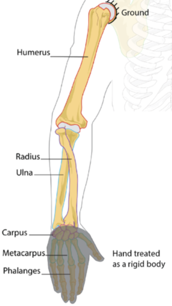
How many dof does the human arm have?
Method 1: add dof of joints (shoulder, elbow, wrist) Method 2: fully constrain hand’s position
Configuration space topology
Consider a point moving on the surface of a sphere. The point’s C-space is two dimensional, as the configuration can be described by two coordinates, latitude and longitude. As another example, a point moving on a plane also has a two-dimensional C-space, with coordinates (x, y). While both a plane and the surface of a sphere are two dimensional, clearly they do not have the same shape – the plane extends infinitely while the sphere wraps around. Unlike the plane, a larger sphere has the same shape as the original sphere, in that it wraps around in the same way. Only its size is different. For that matter, an oval-shaped American football also wraps around similarly to a sphere. The only difference between a football and a sphere is that the football has been stretched in one direction.
The idea that the two-dimensional surfaces of a small sphere, a large sphere, and a football all have the same kind of shape, which is different from the shape of a plane, is expressed by the topology of the surfaces. Example topologies are shown in Figure 5.
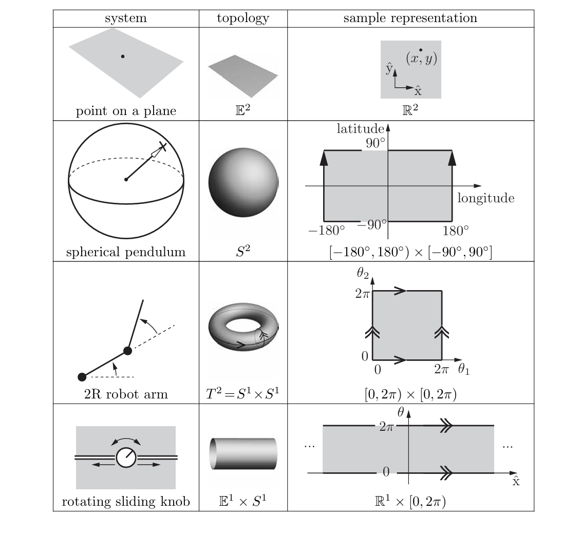
For example, \(S^2\) is the two-dimensional surface of a sphere in three-dimensional space.
since the configuration can be represented as the concatenation of the coordinates (x, y) representing R2 and an angle θ representing S 1 .
The configuration space (C-space) of a rigid body in the plane can be written as \(\mathbb{R}^2 \times S^1\), since the configuration can be represented as the concatenation of the coordinates \((x, y)\), which form \(\mathbb{R}^2\), and an angle \(\theta\), which forms \(S^1\).
The n-dimensional surface of a torus in an (n + 1)-dimensional space. Note that S 1 × S 1 × · · · × S 1 (n copies of S 1 ) is equal to T n , not S n ; for example, a sphere S 2 is not topologically equivalent to a torus T 2.
The configuration space (C-space) of a 2R robot arm can be written as \(S^1 \times S^1 = T^2\), where \(T^n\) is the \(n\)-dimensional surface of a torus in an \((n+1)\)-dimensional space (see Table 2.2). Note that \(S^1 \times S^1 \times \cdots \times S^1\) (with \(n\) copies of \(S^1\)) is equal to \(T^n\), not \(S^n\); for example, a sphere \(S^2\) is not topologically equivalent to a torus \(T^2\).
Note that the topology of a space is a fundamental property of the space itself and is independent of how we choose coordinates to represent points in the space.For example, to represent a point on a circle, we could refer to the point by the angle θ from the center of the circle to the point, relative to a chosen zero angle. Or, we could choose a reference frame with its origin at the center of the circle and represent the point by the two coordinates (x, y) subject to the constraint \(x^2 + y^2 = 1\). No matter what our choice of coordinates is, the space itself does not change.
C-space Representation
Consider the topoplogical space of a sphere as an exmple. One solution for a sphere is to use latitude and longitude coordinates.
In general a choice of \(n\) coordinates, or parameters, to represent an n-dimensional space is called an explicit parametrization of the topology of the space.
A point on the spherical surface can be represented like the well understood coordinates we use for earth navigation:
- Latitude (ϕ): angle from the equator (−90° at South Pole to +90° at North Pole)
- Longitude (λ): angle around the equator (from −180° to +180°)
This coordinate system works well almost everywhere, except at the poles. Imagine you’re very close to the North Pole (ϕ ≈ 90°), and you take a tiny step eastward. Your latitude ϕ barely changes (still near 90°) but your longitude λ may change a lot — even flip from +180° to −180° with just a tiny move.
This means that small physical motions lead to large changes in the coordinates, a situation that is called a singularity that is not a flaw of the sphere itself (which is smooth and uniform), but a limitation of the chosen parametrization. These singularities especially cause problems when computing velocities, because coordinate rates (like \(\dot{\phi}\), \(\dot{\lambda}\)) can become very large or even diverge near the poles, despite the actual speed in 3D space being constant.
To avoid such singularities, we use an implicit representation instead of an explicit parametrization. An implicit representation views the \(n\)-dimensional space as embedded in a Euclidean space of more than \(n\) dimensions, just as a two-dimensional unit sphere can be viewed as a surface embedded in three-dimensional Euclidean space. An implicit representation uses the coordinates of the higher-dimensional space (for example, \((x, y, z)\) in three-dimensional space), but subjects these coordinates to constraints that reduce the number of degrees of freedom. For the unit sphere, the constraint equation is:
\[ x^2 + y^2 + z^2 = 1 \]
A disadvantage of this approach is that the representation involves more variables than the actual number of degrees of freedom, however as it turns out it offers the ability to perform linear operations and therefore its not necessarily computationally inefficient. As we will see the implicit representation of a rotation matrix that encode orientation in 3D space, uses nine numbers subject to three constraints and is a linear operator.
Task space
The task spac is a space in which the robot’s task can be naturally expressed. For example, if the robot’s task is to weld metal, the task space would be limited to \(\mathbb{R}^2\) and obviously the robotic arm has a configuration space topology quite different to the task space.
Workspace
The workspaceis a specification of the configurations that the end-effector of the robot can reach. The definition of the workspace is primarily driven bythe robot’s structure, independently of the task.
References
Lynch and Park, Modern Robotics: Mechanics, Planning, and Control (2017)