Bayesian Inference

The Bayes Rule

Thomas Bayes (1701-1761)

The Bayesian theorem is the cornerstone of probabilistic modeling and ultimately governs what models we can construct inside the learning algorithm. If $\mathbf{w}$ denotes the unknown parameters, $\mathtt{data}$ denotes the dataset and $\mathcal{H}$ denotes the hypothesis set that we met in the learning problem chapter.

$$ p(\mathbf{w} | \mathtt{data}, \mathcal{H}) = \frac{P( \mathtt{data} | \mathbf{w}, \mathcal{H}) P(\mathbf{w} | \mathcal{H}) }{ P( \mathtt{data} | \mathcal{H})} $$

The Bayesian framework allows the introduction of priors $p(\theta | \mathcal{H})$ from a wide variety of sources: experts, other data, past posteriors, etc. It allows us to calculate the posterior distribution from the likelihood function and this prior subject to a normalizing constant.

We will call belief the internal to the agent posterior probability estimate of a random variable as calculated via the Bayes rule.

For example,a medical patient is exhibiting symptoms x, y and z. There are a number of diseases that could be causing all of them, but only a single disease is present. A doctor (the expert) has a belief about the underlying disease, but a second doctor may have a slightly different belief.

Probabilistic Graphical Models

Let us now look at a representation, the probabilistic graphical model (pgm) (also called Bayesian network when the priors are captured) that can be used to capture the structure of such beliefs and in general capture dependencies between the random variables involved in the modeling of a problem. We can use such representations to efficiently compute such beliefs and, in general, compute conditional probabilities. For now we will limit the modeling horizon to just one snapshot in time - later we will expand to capture problems that include time $t$ as a variable.

By convention we represent in PGMs as directed graphs, with nodes being the random variables involved in the model and directed edges indicating a parent child relationship, with the arrow pointing to a child, representing that the child nodes are probabilistically conditioned on the parent(s).

In a hypothetical example of a joint distribution with $K=7$ random variables,

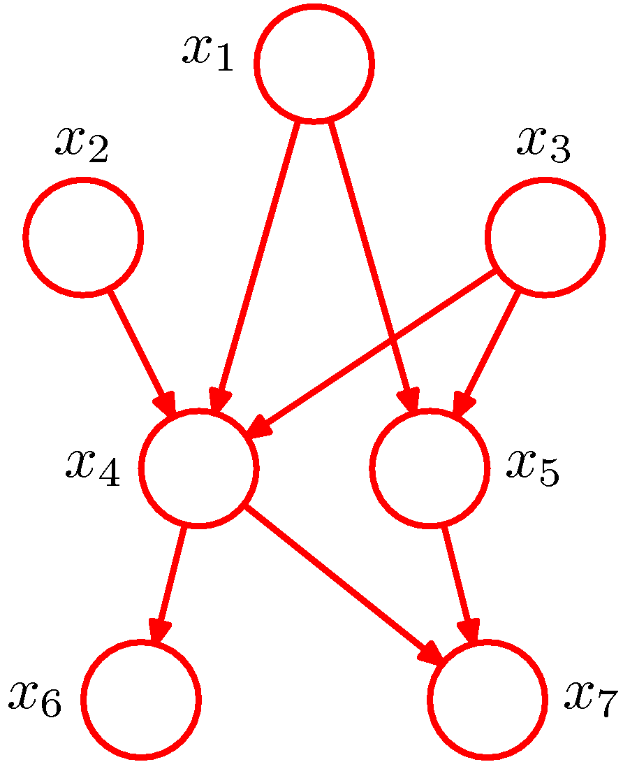
The PGM above represents the joint distribution $p(x_1, x_2, …, x_7)=p(x_1)p(x_2)p(x_3)p(x_4|x_1, x_2, x_3)p(x_5|x_1, x_3) p(x_6|x_4)p(x_7|x_4, x_5)$. In general,

$$p(\mathbf x)= \prod_{k=1}^K p(x_k | \mathtt{pa}_k)$$

where $\mathtt{pa}_k$ is the set of parents of node $x_k$.

Note that we have assumed that our model does not have variables involved in directed cycles and therefore we call such graphs Directed Acyclic Graphs (DAGs).

Bayesian approach vs Maximum Likelihood

In the MLE section we have seen a simple supervised learning problem that is specified via a joint distribution $\hat{p}_{data}(\bm x, y)$ and are asked to fit the model parameterized by the weights $\mathbf w$ using maximum likelihood. Its important to view pictorially perhaps the most important effect of Bayesian thinking in the regression setting:

• The $\mathbf{w}$ in MLE is a point estimate $\mathbf{w}_{MLE}$ and we are plugging this estimate in the predictive distribution to make predictions $\hat y$ for data we havent seen before.

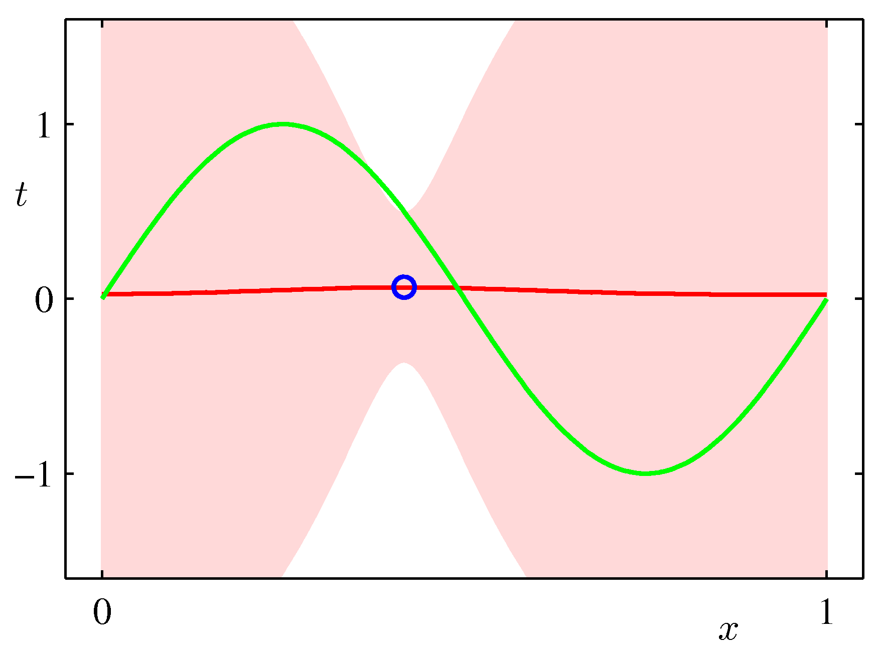
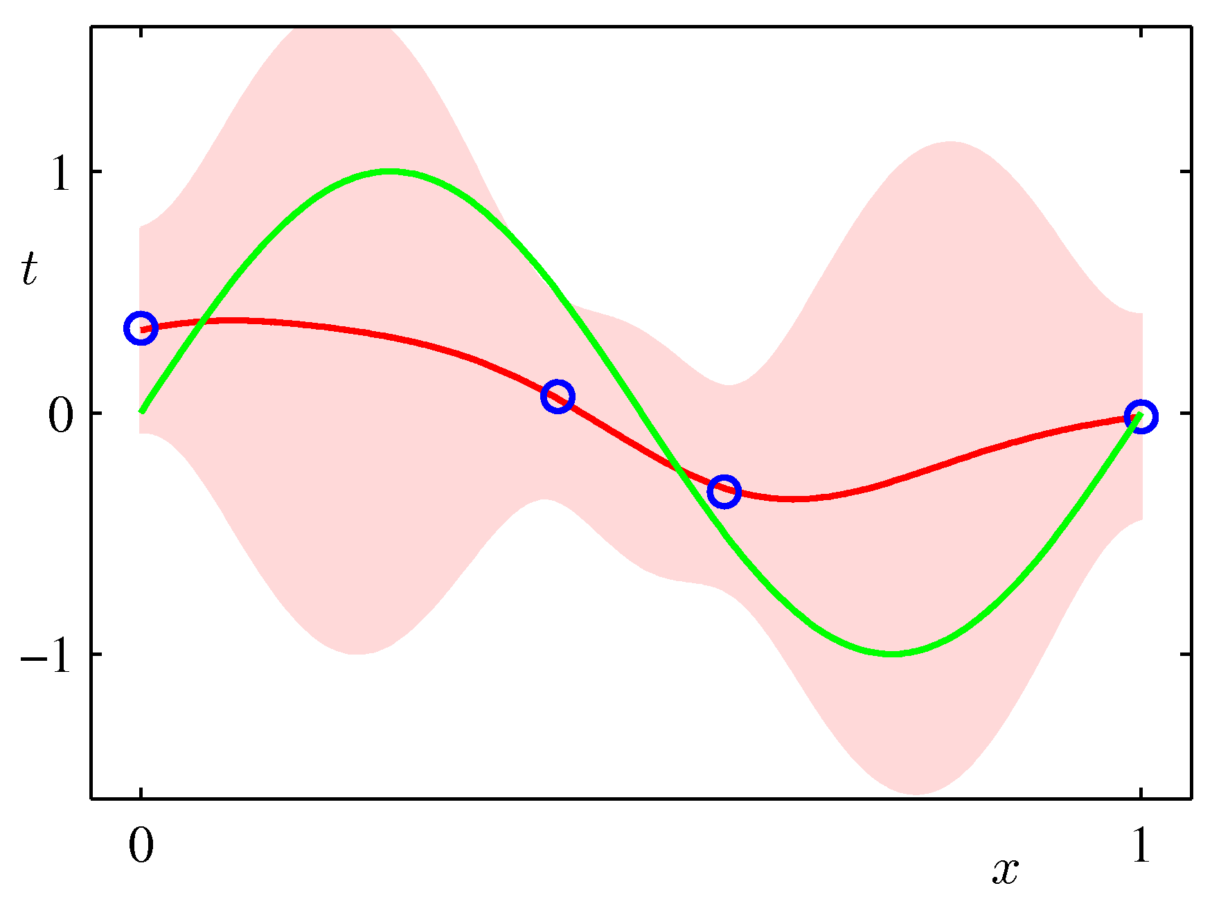
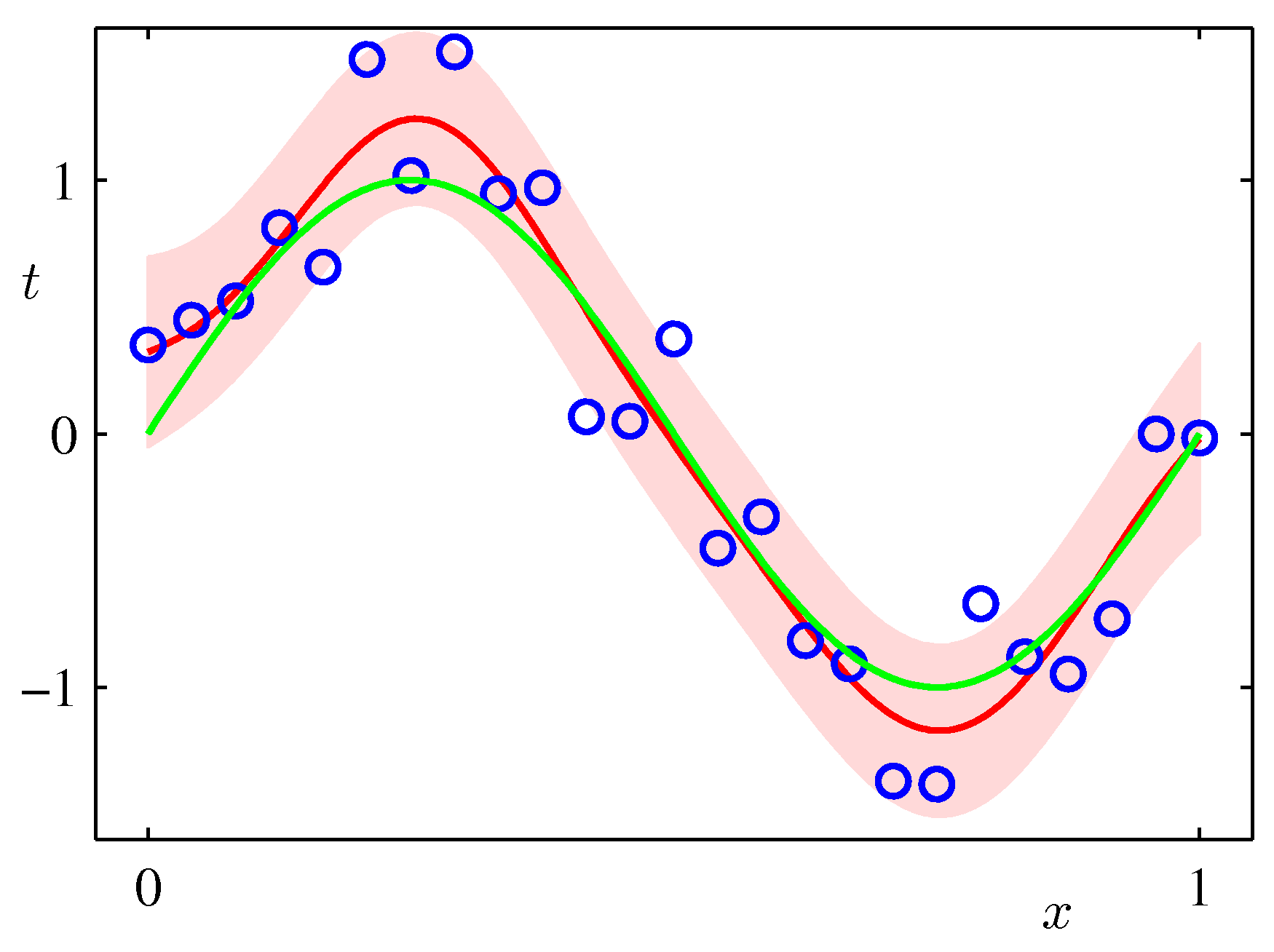
• In the Bayesian setting on the other hand we use a full distribution over $\mathbf w$. We predict by integrating over the posterior of $\mathbf{w}$ (i.e. given the data) and therefore considering organically the uncertainty of the posterior of $\mathbf{w}$ in our predictions. As such it can capture the effects of sparse data producing more uncertainty via its covariance in areas where there are no data as shown in the following example which is exactly the same sinusoidal dataset fit with Bayesian updates and Gaussian basis functions.

ML frameworks have been enhanced recently to deal with Bayesian approaches and approximations that make such approaches feasible for both classical and deep learning. TF.Probability and PyTorch Pyro are examples of such enhancements.

Before diving into the posterior update in regression problems its instructive to go over the Bayesian coin tossing notebook that shows a simpler experiment.

Online Bayesian Regression

Lets us consider an instructive example of applying the Bayesian approach in an online learning setting (streaming data arriving over the wire). In this example where the underlying target function is $p_{data}(x, \mathbf w) = w_0 + w_1 x + n$ This is the equation of a line. In this example its parametrized with $a_0=-0.3, a_1=0.5$ and $n \in \mathcal N(0, \sigma=0.2)$. To match the simple inference exercise that we just saw, we draw the equivalent PGM

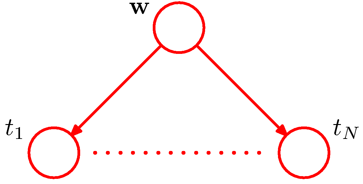
Bayesian Linear Regression example - please replace $t$ with $y$ to match earlier notation in these notes

The Bayesian update of the posterior can be intuitively understood using a graphical example of our model of the form: $$g(x,\mathbf{w})= w_0 + w_1 x$$ (our hypothesis). The reason why we pick this example is illustrative as the model has just two parameters and is amendable to visualization. The update needs a prior distribution over $\mathbf w$ and a likelihood function. As prior we assume a spherical Gaussian

$$p(\mathbf w | \alpha) = \mathcal N(\mathbf w | \mathbf 0, \alpha^{-1} \mathbf I)$$

with $\alpha = 0.2$. We starts in row 1 with this prior and at this point there are no data and the likelihood is undefined while every possible linear (line) hypothesis is feasible as represented by the red lines. In row 2, a data point arrives and the the Bayesian update takes place: the previous row posterior becomes the prior and is multiplied by the current likelihood function. The likelihood function and the form of the math behind the update are as shown in Bishop’s book in section 3.3. Here we focus on a pictorial view of what is the update is all about and how the estimate of the posterior distribution $p(\mathbf w | \mathbf y)$ ultimately (as the iterations increase) it will be ideally centered to the ground truth ($\bm a$).

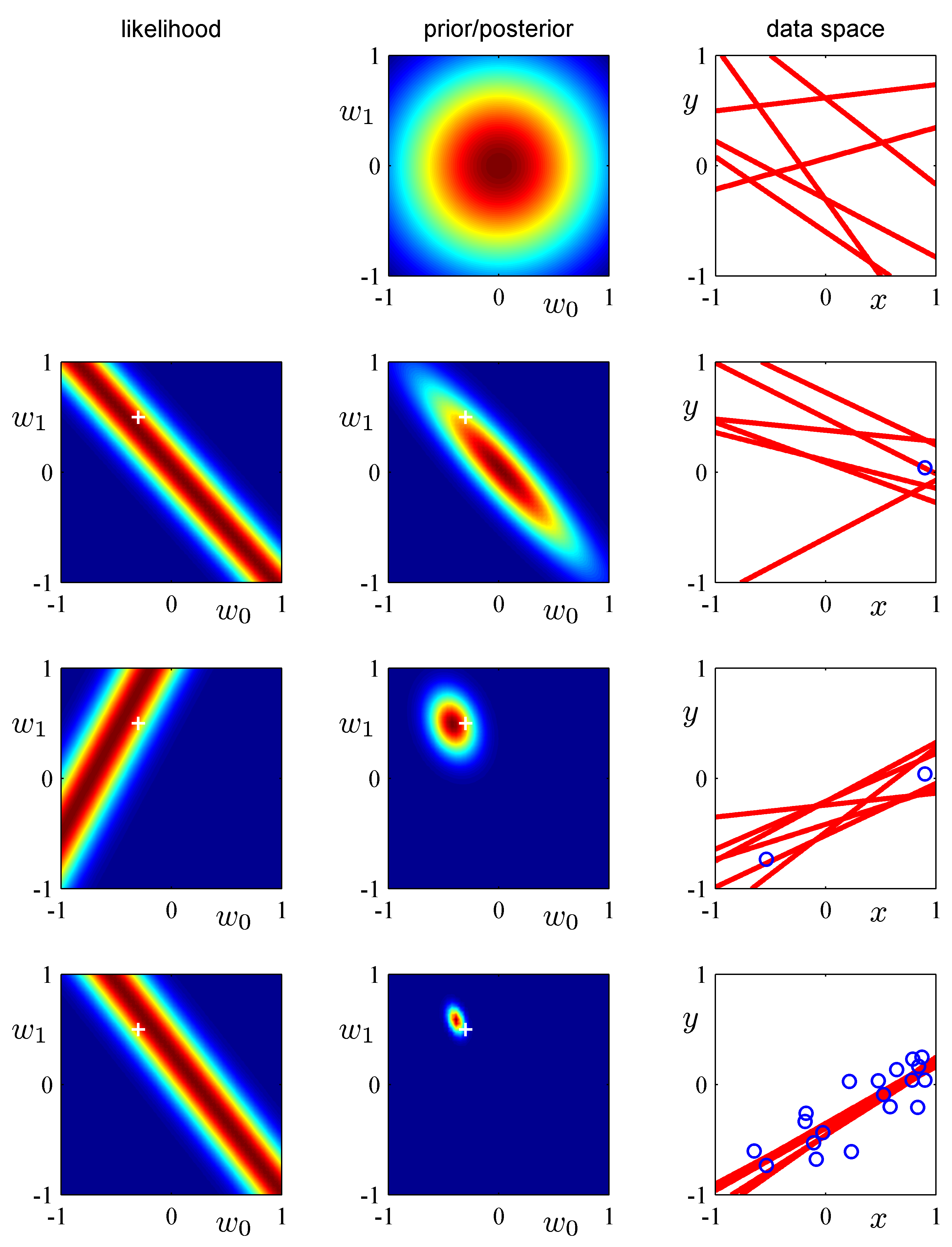Instructive example of Bayesian learning as data points are streamed into the learner. Notice the dramatic improvement in the posterior the moment the 2nd data point arrives. Why is that?

Bayesian Regression implementation

Notice in the notebook the two of the three broad benefits of the Bayesian approach:

• Compatibility with online learning - online learning does not mean necessarily that the data arrive over the ‘wire’ but it means that we can consider few data at a time.
• Adjustment of the predictive uncertainty (cov) to the sparsity of the data.
• Incorporation of external beliefs / opinions that can be naturally expressed probabilistically.