Entropy

In this section we take a closer look into the algorithm block of the learning problem. This block implements the underlying optimization problem that produces the weights in regression and classification settings. Any optimization problem requires an objective function and as it turns out in the supervised setting (and not only) there is a whole theory, called information theory pioneered by Claude Shannon at Bell Labs, that guides us in our search to find the best $p_{model}$ but also in a myriad other things. The important elements of this theory are reviewed here.

Value of information: Low Manhattan-bound traffic flow in Holland tunnel on Monday morning

An outcome $x_t$ carries information that is a function of the probability of this outcome $P(x_t)$ by,

$I(x_t) = \ln \frac{1}{P(x_t)} = - \ln P(x_t)$

This can be intuitively understood when you compare two outcomes. For example, consider someone is producing the result of the vehicular traffic flow outside of Holland tunnel on Monday morning. The information that the results is “low” carries much more information when the result is “high” since most people expect that there will be horrendous traffic going into Manhattan on Monday mornings. When we want to represent the amount of uncertainty over a distribution (i.e. the traffic in Holland tunnel over all times) we can take the expectation over all possible outcomes i.e.

$H(P) = - \mathbb{E} \ln P(x)$

and we call this quantity the entropy of the probability distribution $P(x)$. When $x$ is continuous the entropy is known as differential entropy. Continuing the alphabetical example, we can determine the entropy over the distribution of letters in the sample text we met before as,

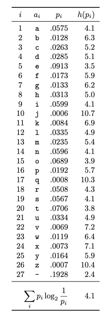
This is 4.1 bits (as the $\log$ is taken with base 2). This represents the average number of bits required to transmit each letter of this text to a hypothetical receiver. Note that we used the information carried by each “outcome” (the letter) that our source produced. If the source was binary, we can plot the entropy of such source over the probability p that the outcome is a 1 as shown below,

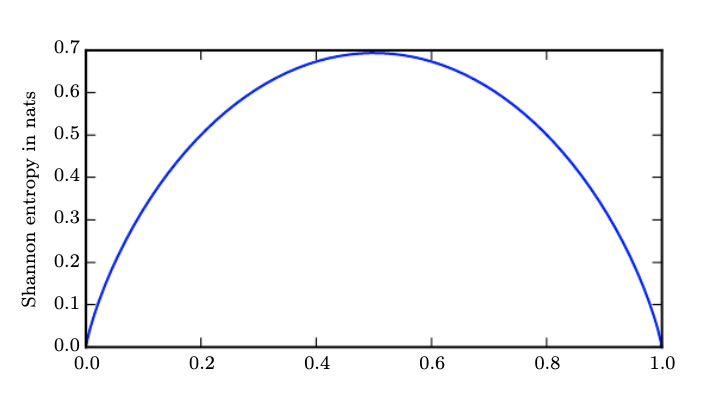
The plot simply was produced by taking the definition of entropy and applying to the binary case,

$H(p) = - [p \ln p + (1-p) \ln(1-p)]$

As you can see the maximum entropy is when the outcome is most unpredictable i.e. when a 1 can show up with uniform probability (in this case equal probability to a 0). Entropy has widespread implications as it measures our uncertainty in terms of the length of the message/code that we need to communicate the outcome across. Taking to the limit if we were certain about an event (deterministic outcome) we would need 0 bits or require to send any message at all.

Relative entropy or KL divergence

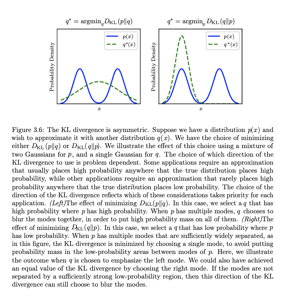
In many settings we need to have a metric that compares two probability distributions ${P(x),Q(x)}$ in terms of their “distance” from each other (the quotes will be explained shortly). This is given by the quantity known as relative entropy or KL divergence.

$$KL(P||Q)= \mathbb{E}[\ln P(x) - \ln Q(x)]$$

If the two distributions are identical, $KL=0$ - in general however $KL(P||Q) \ge 0$. One key element to understand is that $KL$ is not a true distance metric as its asymmetric.

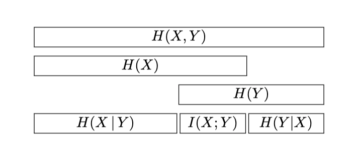
Very close to the relative entropy is probably one of the most used information theoretic concepts in ML: the cross-entropy. We will motivate cross entropy via a diagram shown below,

Digging further

If you are a visual learner, the visual information theory blog post is a better starting point to the above. MacKay’s book (Chapter 2) is an instructive introduction to probability and information theory concepts and you can test your understanding by doing the exercises in that chapter.