Logistic Regression

Logistic regression is used in machine learning extensively - every time we need to provide probabilistic semantics to an outcome e.g. predicting the risk of developing a given disease (e.g. diabetes; coronary heart disease), based on observed characteristics of the patient (age, sex, body mass index, results of various blood tests, etc.), whether an voter will vote for a given party, predicting the probability of failure of a given process, system or product, predicting a customer’s propensity to purchase a product or halt a subscription, predicting the likelihood of a homeowner defaulting on a mortgage.

Odds and the Logistic Sigmoid

If $\sigma$ is a probability of an event, then the ratio $\frac{\sigma}{1-\sigma}$ is the corresponding odds, the ratio of the event occurring divided by not occurring. For example, if a race horse runs 100 races and wins 25 times and loses the other 75 times, the probability of winning is 25/100 = 0.25 or 25%, but the odds of the horse winning are 25/75 = 0.333 or 1 win to 3 loses. In the binary classification case, the log odds is given by

$$ \mathtt{logit}(\sigma) = \alpha = \ln \frac{\sigma}{1-\sigma} = \ln \frac{p(\mathcal{C}_1|\mathbf{x})}{p(\mathcal{C}_2|\mathbf{x})}$$

What is used in ML though is the logistic function of any number $\alpha$ that is given by the inverse logit:

$$\mathtt{logistic}(\alpha) = \sigma(\alpha) = \mathtt{logit}^{-1}(\alpha) = \frac{1}{1 + \exp(-\alpha)} = \frac{\exp(\alpha)}{ \exp(\alpha) + 1}$$

and is plotted below. It maps its argument to the “probability” space [0,1].

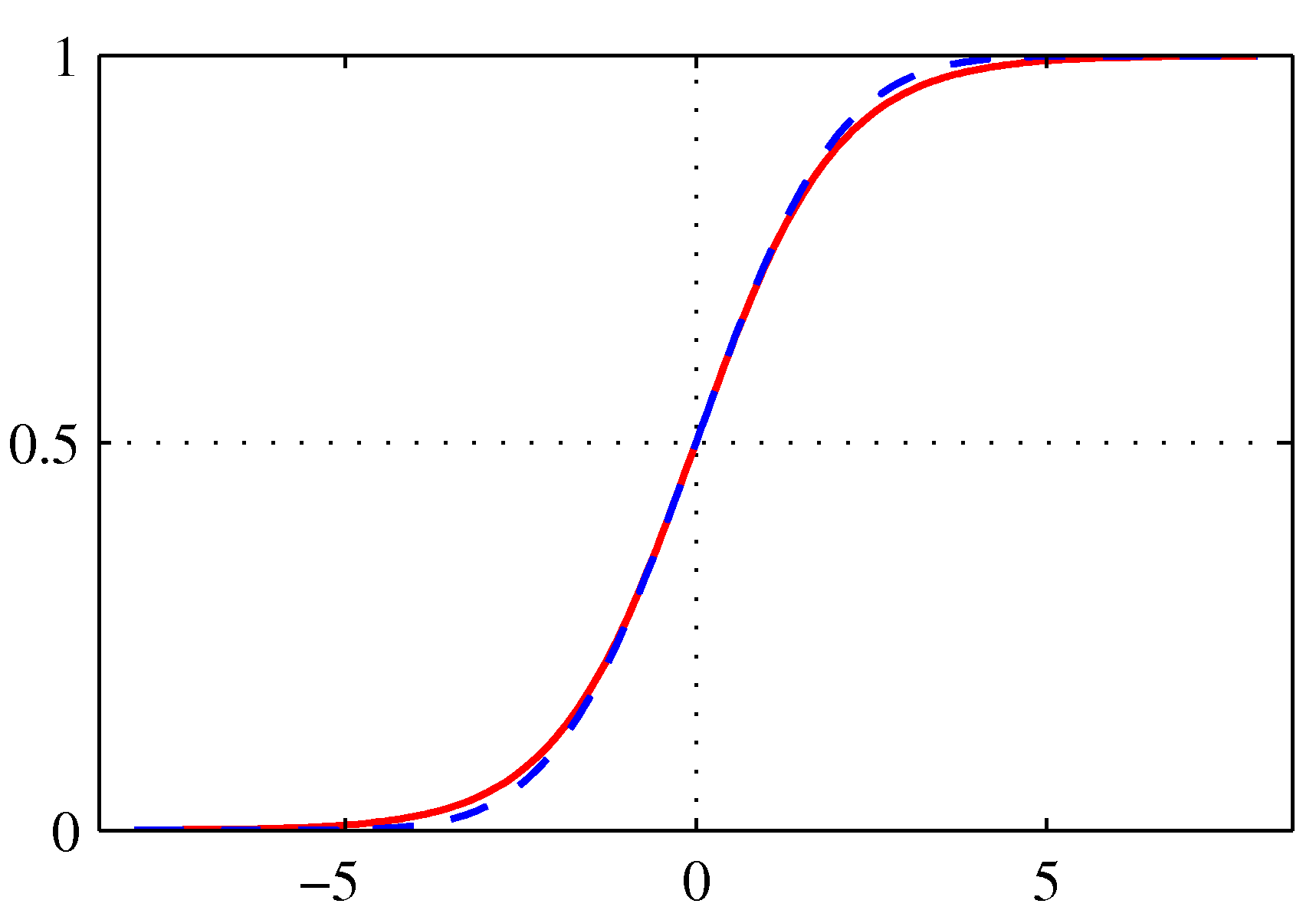Logistic sigmoid (red)

The sigmoid function satisfies the following symmetry:

$$\sigma(-\alpha) = 1 - \sigma(\alpha)$$

Binary case

If we consider the two class problem, we can write the posterior probability as,

$$p(\mathcal{C}_1|\mathbf{x}) = \frac{p(\mathbf{x}|\mathcal{C}_1) p(\mathcal{C}_1)}{p(\mathbf{x}|\mathcal{C}_1) p(\mathcal{C}_1) + p(\mathbf{x}|\mathcal{C}_2) p(\mathcal{C}_2)} = \frac{1}{1 + \exp(-\alpha)} = \sigma(\alpha)$$

where $\alpha = \ln \frac{p(\mathbf{x}|\mathcal{C}_1) p(\mathcal{C}_1)}{p(\mathbf{x}|\mathcal{C}_2) p(\mathcal{C}_2)}$.

Given the posterior distribution above we have for the specific linear activation,

$$p(\mathcal{C}_1|\mathbf{x}) = \sigma(\mathbf{w}^T \mathbf{x})$$

This model is what statisticians call logistic regression - despite its name its a model for classification.

The figure below shows the corresponding posterior distribution $p(\mathcal{C}_1|\mathbf{x})$

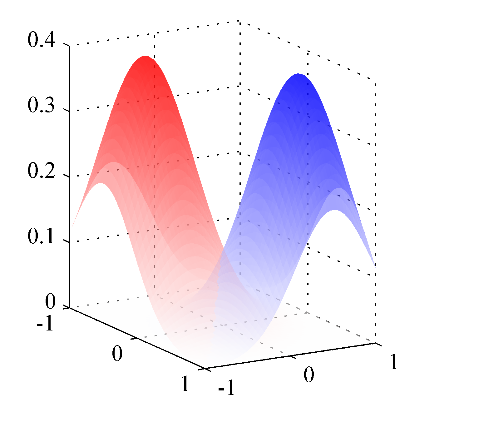The class-conditional densities for two classes, denoted red and blue. Here the class-conditional densities $p(\mathbf{x}|\mathcal{C}_1)$ and $p(\mathbf{x}|\mathcal{C}_2)$ are Gaussian

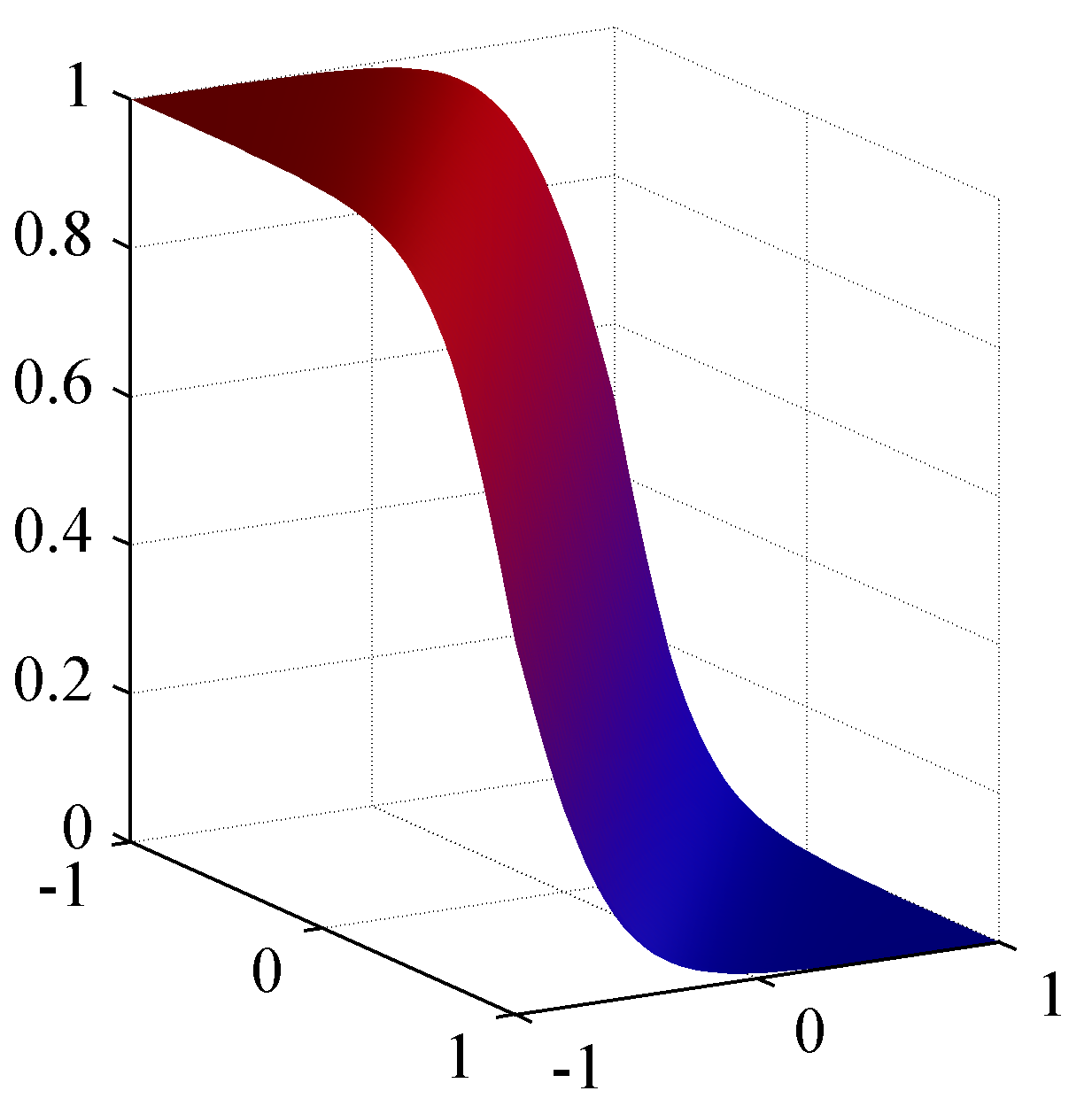The corresponding posterior probability for the red class, which is given by a logistic sigmoid of a linear function of $\mathbf{x}$.

By repeating the classical steps in ML methodology i.e. writing down the expression of the likelihood function (this will now be a product of binomials), we can write down the negative log likelihood function for the binary case as,

$$L(\mathbf{w}) = L(y, \hat{y}) = - \ln p(\mathbf{y},\mathbf{w}) = - \big[ \sum_{i=1}^m {y_i \ln \hat{y}_i + (1-y_i) \ln (1-\hat{y}_i) } \big]$$

which is called cross entropy loss function - probably the most widely used error function (in classification as well as regression) due to its information theoretic roots.

Its shape is shown in the figure below for an example case where the $y=1$. It is also known as log-loss.

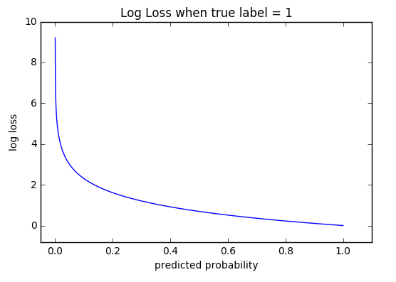
CE Loss vs predicted probability for class “1”

The behavior of the loss function is telling: it heavily penalizes confident wrong decisions. Notice its exponential rise when the probability $\hat{y}$ of the class “1” is close to 0.0 which means that the classifier predicted with high confidence the opposite class that the ground truth. On the other hand, when the probability of $\hat y$ is close to 1.0, which means that the classifier predicts the class “1” with confidence, we exhibit minimal loss and in the limit zero loss.

Minimizing the error function with respect to $\mathbf{w}$ requires calculating its gradient,

$$\nabla L = \sum_{i=1}^m (\hat{y}_i - y_i) x_i$$

The expression above defines the batch gradient decent algorithm. We can then readily convert this algorithm to SGD by considering mini-batch updates for any mini-batch size (usually delegated as a hyperparameter).