The whitening operator

Some of material in this section have been borrowed from CS231n

Designing and training a network using SGD and backprop requires making seemingly arbitrary choices such as the types and number of neurons, layers, learning rates, training and test datasets etc. These choices can be critical yet there is no full proof recipe for deciding them because they are naturally problem and data dependent. However there are heuristics and some underlying theory that can help a practitioner to make better choices.

Perhaps one of the most important methods for accelerating training as described in this paper is the whitening operation. We describe the operation first and then couple it to the training process in a dedicated section.

This operation involves three main steps as described next.

Preprocessing

There are three common forms of data preprocessing a data matrix $X$, where we will assume that $X$ is of size $[m \times n]$ ($m$ is the number of data, $n$ is their dimensionality).

Translation by mean subtraction is the most common form of preprocessing. It involves subtracting the mean across every individual feature in the data, and has the geometric interpretation of centering the cloud of data around the origin along every dimension. In numpy, this operation would be implemented as: X -= np.mean(X, axis = 0).

Normalization refers to normalizing the data dimensions so that they are of approximately the same scale. There are two common ways of achieving this normalization. One is to divide each dimension by its standard deviation, once it has been zero-centered: X /= np.std(X, axis = 0). Another form of this preprocessing normalizes each dimension so that the min and max along the dimension is -1 and 1 respectively. It only makes sense to apply this preprocessing if you have a reason to believe that different input features have different scales (or units), but they should be of approximately equal importance to the learning algorithm.

Common data preprocessing pipeline. Left: Original toy, 2-dimensional input data. Middle: The data is zero-centered by subtracting the mean in each dimension. The data cloud is now centered around the origin. Right: Each dimension is additionally scaled by its standard deviation. The red lines indicate the extent of the data - they are of unequal length in the middle, but of equal length on the right.

Decorrelative Projection

In this process, the data is first centered as described above. Then, we can compute the covariance matrix that tells us about the correlation structure in the data:

1
2
3

# Assume input data matrix X of size [m x n]
X -= np.mean(X, axis = 0) # zero-center the data (important)
cov = np.dot(X.T, X) / X.shape[0] # get the data covariance matrix

The (i,j) element of the data covariance matrix contains the covariance between i-th and j-th dimension of the data. In particular, the diagonal of this matrix contains the variances. Furthermore, the covariance matrix is symmetric and positive semi-definite. We can compute the SVD factorization of the data covariance matrix:

1

U,S,V = np.linalg.svd(cov)

where the columns of $U$ are the eigenvectors and $S$ is a 1-D array of the singular values. To decorrelate the data, we project the original (but zero-centered) data into the eigenbasis:

1

Xrot = np.dot(X, U) # decorrelate the data

Notice that the columns of $U$ are a set of orthonormal vectors (norm of 1, and orthogonal to each other), so they can be regarded as basis vectors. The projection therefore corresponds to a rotation of the data in $X$ so that the new axes are the eigenvectors. If we were to compute the covariance matrix of $Xrot$, we would see that it is now diagonal.

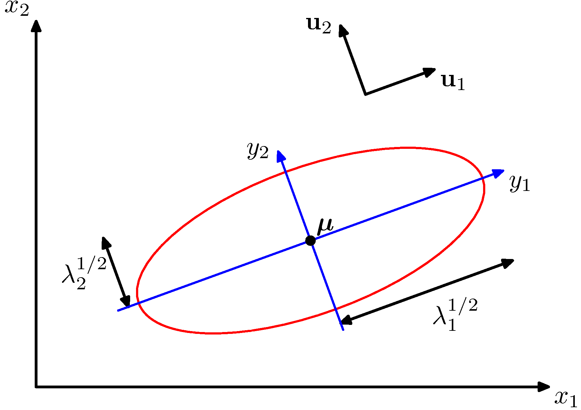Bivariate Gaussian and its eigen-directions (new coordinate system)

A nice property of np.linalg.svd is that in its returned value $U$, the eigenvector columns are sorted by their eigenvalues. We can use this to reduce the dimensionality of the data by only using the top few eigenvectors, and discarding the dimensions along which the data has no variance. This is also sometimes refereed to as Principal Component Analysis (PCA) dimensionality reduction:

1

Xrot_reduced = np.dot(X, U[:,:100]) # Xrot_reduced becomes [m x 100]

After this operation, we would have reduced the original dataset of size [m x n] to one of size [m x 100], keeping the 100 dimensions of the data that contain the most variance. It is very often the case that you can get very good performance by training linear classifiers or neural networks on the PCA-reduced datasets, obtaining savings in both space and time.

Whitening

The whitening operation takes the data in the eigenbasis and divides every dimension by the eigenvalue to normalize the scale. The geometric interpretation of this transformation is that if the input data is a multivariable gaussian, then the whitened data will be a gaussian with zero mean and identity covariance matrix. This step would take the form:

1
2
3

# whiten the data:
# divide by the eigenvalues (which are square roots of the singular values)
Xwhite = Xrot / np.sqrt(S + 1e-5)

Left: Original toy, 2-dimensional input data. Middle: After performing PCA. The data is centered at zero and then rotated into the eigenbasis of the data covariance matrix. This decorrelates the data (the covariance matrix becomes diagonal). Right: Each dimension is additionally scaled by the eigenvalues, transforming the data covariance matrix into the identity matrix. Geometrically, this corresponds to stretching and squeezing the data into an isotropic gaussian blob.

We can also try to visualize these transformations with CIFAR-10 images. The training set of CIFAR-10 is of size 50,000 x 3072, where every image is stretched out into a 3072-dimensional row vector. We can then compute the [3072 x 3072] covariance matrix and compute its SVD decomposition (which can be relatively expensive). What do the computed eigenvectors look like visually? An image might help:

Left:An example set of 49 images. 2nd from Left: The top 144 out of 3072 eigenvectors. The top eigenvectors account for most of the variance in the data, and we can see that they correspond to lower frequencies in the images. 2nd from Right: The 49 images reduced with PCA, using the 144 eigenvectors shown here. That is, instead of expressing every image as a 3072-dimensional vector where each element is the brightness of a particular pixel at some location and channel, every image above is only represented with a 144-dimensional vector, where each element measures how much of each eigenvector adds up to make up the image. In order to visualize what image information has been retained in the 144 numbers, we must rotate back into the “pixel” basis of 3072 numbers. Since U is a rotation, this can be achieved by multiplying by U.transpose()[:144,:], and then visualizing the resulting 3072 numbers as the image. You can see that the images are slightly blurrier, reflecting the fact that the top eigenvectors capture lower frequencies. However, most of the information is still preserved. Right: Visualization of the “white” representation, where the variance along every one of the 144 dimensions is squashed to equal length. Here, the whitened 144 numbers are rotated back to image pixel basis by multiplying by U.transpose()[:144,:]. The lower frequencies (which accounted for most variance) are now negligible, while the higher frequencies (which account for relatively little variance originally) become exaggerated.

Common pitfall. An important point to make about the preprocessing is that any preprocessing statistics (e.g. the data mean) must only be computed on the training data, and then applied to the validation / test data. e.g. computing the mean and subtracting it from every image across the entire dataset and then splitting the data into train/val/test splits would be a mistake. Instead, the mean must be computed only over the training data and then subtracted equally from all splits (train/val/test). In other words whatever preprocessing we do to the training data, it has to be applied to validation and test data identically.