  1
  2
  3
  4
  5
  6
  7
  8
  9
 10
 11
 12
 13
 14
 15
 16
 17
 18
 19
 20
 21
 22
 23
 24
 25
 26
 27
 28
 29
 30
 31
 32
 33
 34
 35
 36
 37
 38
 39
 40
 41
 42
 43
 44
 45
 46
 47
 48
 49
 50
 51
 52
 53
 54
 55
 56
 57
 58
 59
 60
 61
 62
 63
 64
 65
 66
 67
 68
 69
 70
 71
 72
 73
 74
 75
 76
 77
 78
 79
 80
 81
 82
 83
 84
 85
 86
 87
 88
 89
 90
 91
 92
 93
 94
 95
 96
 97
 98
 99
100
101
102
103
104
105
106
107
108
109
110
111
112
113
114
115
116
117
118
119
120
|
"""Contains model definitions for versions of the Oxford VGG network.
These model definitions were introduced in the following technical report:
  Very Deep Convolutional Networks For Large-Scale Image Recognition
  Karen Simonyan and Andrew Zisserman
  arXiv technical report, 2015
  PDF: http://arxiv.org/pdf/1409.1556.pdf
  ILSVRC 2014 Slides: http://www.robots.ox.ac.uk/~karen/pdf/ILSVRC_2014.pdf
  CC-BY-4.0
More information can be obtained from the VGG website:
www.robots.ox.ac.uk/~vgg/research/very_deep/
Usage:
  with slim.arg_scope(vgg.vgg_arg_scope()):
    outputs, end_points = vgg.vgg_a(inputs)
  with slim.arg_scope(vgg.vgg_arg_scope()):
    outputs, end_points = vgg.vgg_16(inputs)
@@vgg_16

"""
from __future__ import absolute_import
from __future__ import division
from __future__ import print_function

import tensorflow.compat.v1 as tf
import tf_slim as slim

def vgg_arg_scope(weight_decay=0.0005):
  """Defines the VGG arg scope.
  Args:
    weight_decay: The l2 regularization coefficient.
  Returns:
    An arg_scope.
  """
  with slim.arg_scope([slim.conv2d, slim.fully_connected],
                      activation_fn=tf.nn.relu,
                      weights_regularizer=slim.l2_regularizer(weight_decay),
                      biases_initializer=tf.zeros_initializer()):
    with slim.arg_scope([slim.conv2d], padding='SAME') as arg_sc:
      return arg_sc

def vgg_16(inputs,
           num_classes=1000,
           is_training=True,
           dropout_keep_prob=0.5,
           spatial_squeeze=True,
           reuse=None,
           scope='vgg_16',
           fc_conv_padding='VALID',
           global_pool=False):
  """Oxford Net VGG 16-Layers version D Example.
  Note: All the fully_connected layers have been transformed to conv2d layers.
        To use in classification mode, resize input to 224x224.
  Args:
    inputs: a tensor of size [batch_size, height, width, channels].
    num_classes: number of predicted classes. If 0 or None, the logits layer is
      omitted and the input features to the logits layer are returned instead.
    is_training: whether or not the model is being trained.
    dropout_keep_prob: the probability that activations are kept in the dropout
      layers during training.
    spatial_squeeze: whether or not should squeeze the spatial dimensions of the
      outputs. Useful to remove unnecessary dimensions for classification.
    reuse: whether or not the network and its variables should be reused. To be
      able to reuse 'scope' must be given.
    scope: Optional scope for the variables.
    fc_conv_padding: the type of padding to use for the fully connected layer
      that is implemented as a convolutional layer. Use 'SAME' padding if you
      are applying the network in a fully convolutional manner and want to
      get a prediction map downsampled by a factor of 32 as an output.
      Otherwise, the output prediction map will be (input / 32) - 6 in case of
      'VALID' padding.
    global_pool: Optional boolean flag. If True, the input to the classification
      layer is avgpooled to size 1x1, for any input size. (This is not part
      of the original VGG architecture.)
  Returns:
    net: the output of the logits layer (if num_classes is a non-zero integer),
      or the input to the logits layer (if num_classes is 0 or None).
    end_points: a dict of tensors with intermediate activations.
  """
  with tf.variable_scope(
      scope, 'vgg_16', [inputs], reuse=reuse) as sc:
    end_points_collection = sc.original_name_scope + '_end_points'
    # Collect outputs for conv2d, fully_connected and max_pool2d.
    with slim.arg_scope([slim.conv2d, slim.fully_connected, slim.max_pool2d],
                        outputs_collections=end_points_collection):
      net = slim.repeat(inputs, 2, slim.conv2d, 64, [3, 3], scope='conv1')
      net = slim.max_pool2d(net, [2, 2], scope='pool1')
      net = slim.repeat(net, 2, slim.conv2d, 128, [3, 3], scope='conv2')
      net = slim.max_pool2d(net, [2, 2], scope='pool2')
      net = slim.repeat(net, 3, slim.conv2d, 256, [3, 3], scope='conv3')
      net = slim.max_pool2d(net, [2, 2], scope='pool3')
      net = slim.repeat(net, 3, slim.conv2d, 512, [3, 3], scope='conv4')
      net = slim.max_pool2d(net, [2, 2], scope='pool4')
      net = slim.repeat(net, 3, slim.conv2d, 512, [3, 3], scope='conv5')
      net = slim.max_pool2d(net, [2, 2], scope='pool5')

      # Use conv2d instead of fully_connected layers.
      net = slim.conv2d(net, 4096, [7, 7], padding=fc_conv_padding, scope='fc6')
      net = slim.dropout(net, dropout_keep_prob, is_training=is_training,
                         scope='dropout6')
      net = slim.conv2d(net, 4096, [1, 1], scope='fc7')
      # Convert end_points_collection into a end_point dict.
      end_points = slim.utils.convert_collection_to_dict(end_points_collection)
      if global_pool:
        net = tf.reduce_mean(
            input_tensor=net, axis=[1, 2], keepdims=True, name='global_pool')
        end_points['global_pool'] = net
      if num_classes:
        net = slim.dropout(net, dropout_keep_prob, is_training=is_training,
                           scope='dropout7')
        net = slim.conv2d(net, num_classes, [1, 1],
                          activation_fn=None,
                          normalizer_fn=None,
                          scope='fc8')
        if spatial_squeeze:
          net = tf.squeeze(net, [1, 2], name='fc8/squeezed')
        end_points[sc.name + '/fc8'] = net
      return net, end_points
vgg_16.default_image_size = 224

# Alias
vgg_d = vgg_16
|

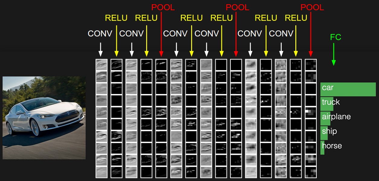
 VGG Configurations: Different columns represent different depths
 VGG16 Network
 GradCAM block diagram
 Results of GradCAM for ResNet50 training on ImageNet_