# Imports
import copy
import matplotlib.pyplot as plt
import numpy as np
import os
import time

plt.ion()Quantized Transfer Learning for Computer Vision Tutorial
Author: Zafar Takhirov
Reviewed by: Raghuraman Krishnamoorthi
Edited by: Jessica Lin
This tutorial builds on the original PyTorch Transfer Learning tutorial, written by Sasank Chilamkurthy. Transfer learning refers to techniques that make use of a pretrained model for application on a different data-set. There are two main ways the transfer learning is used: 1. ConvNet as a fixed feature extractor: Here, you “freeze” the weights of all the parameters in the network except that of the final several layers (aka “the head”, usually fully connected layers). These last layers are replaced with new ones initialized with random weights and only these layers are trained. 2. Finetuning the ConvNet: Instead of random initializaion, the model is initialized using a pretrained network, after which the training proceeds as usual but with a different dataset. Usually the head (or part of it) is also replaced in the network in case there is a different number of outputs. It is common in this method to set the learning rate to a smaller number. This is done because the network is already trained, and only minor changes are required to “finetune” it to a new dataset.
You can also combine the above two methods: First you can freeze the feature extractor, and train the head. After that, you can unfreeze the feature extractor (or part of it), set the learning rate to something smaller, and continue training.
In this part you will use the first method – extracting the features using a quantized model.
Part 0. Prerequisites
Before diving into the transfer learning, let us review the “prerequisites”, such as installations and data loading/visualizations.
Installing the Nightly Build
Because you will be using the experimental parts of the PyTorch, it is recommended to install the latest version of torch and torchvision. You can find the most recent instructions on local installation here. For example, to install without GPU support:
   pip install numpy
   pip install --pre torch torchvision -f https://download.pytorch.org/whl/nightly/cpu/torch_nightly.html
# For CUDA support use https://download.pytorch.org/whl/nightly/cu101/torch_nightly.html!yes y | pip uninstall torch torchvision
!yes y | pip install --pre torch torchvision -f https://download.pytorch.org/whl/nightly/cu101/torch_nightly.htmlUninstalling torch-1.3.1:
Would remove:
/usr/local/bin/convert-caffe2-to-onnx
/usr/local/bin/convert-onnx-to-caffe2
/usr/local/lib/python3.6/dist-packages/caffe2/*
/usr/local/lib/python3.6/dist-packages/torch-1.3.1.dist-info/*
/usr/local/lib/python3.6/dist-packages/torch/*
Proceed (y/n)? y
y
y
Successfully uninstalled torch-1.3.1
Uninstalling torchvision-0.4.2:
Would remove:
/usr/local/lib/python3.6/dist-packages/torchvision-0.4.2.dist-info/*
/usr/local/lib/python3.6/dist-packages/torchvision/*
Proceed (y/n)? Successfully uninstalled torchvision-0.4.2
Looking in links: https://download.pytorch.org/whl/nightly/cu101/torch_nightly.html
Collecting torch
Downloading https://download.pytorch.org/whl/nightly/cu101/torch-1.4.0.dev20191206-cp36-cp36m-linux_x86_64.whl (897.6MB)
|█████████████████████████████▊ | 834.1MB 67.9MB/s eta 0:00:01tcmalloc: large alloc 1147494400 bytes == 0x38b30000 @ 0x7f396999b615 0x592727 0x4cc529 0x4cc68b 0x50a94c 0x50c5b9 0x508245 0x50a080 0x50aa7d 0x50c5b9 0x508245 0x50a080 0x50aa7d 0x50d390 0x58ef53 0x50c810 0x58ef53 0x50c810 0x58ef53 0x50c810 0x58ef53 0x5f80a2 0x4e5ba3 0x551b81 0x5aa6ec 0x50abb3 0x50d390 0x509d48 0x50aa7d 0x50c5b9 0x508245
|████████████████████████████████| 897.6MB 20kB/s
Collecting torchvision
Downloading https://download.pytorch.org/whl/nightly/cu101/torchvision-0.5.0.dev20191206-cp36-cp36m-linux_x86_64.whl (4.1MB)
|████████████████████████████████| 4.1MB 55.1MB/s
Requirement already satisfied: six in /usr/local/lib/python3.6/dist-packages (from torchvision) (1.12.0)
Requirement already satisfied: numpy in /usr/local/lib/python3.6/dist-packages (from torchvision) (1.17.4)
Requirement already satisfied: pillow>=4.1.1 in /usr/local/lib/python3.6/dist-packages (from torchvision) (4.3.0)
Requirement already satisfied: olefile in /usr/local/lib/python3.6/dist-packages (from pillow>=4.1.1->torchvision) (0.46)
Installing collected packages: torch, torchvision
Successfully installed torch-1.4.0.dev20191206 torchvision-0.5.0.dev20191206Load Data
Note: This section is identical to the original transfer learning tutorial. We will use torchvision and torch.utils.data packages to load the data.
The problem you are going to solve today is classifying ants and bees from images. The dataset contains about 120 training images each for ants and bees. There are 75 validation images for each class. This is considered a very small dataset to generalize on. However, since we are using transfer learning, we should be able to generalize reasonably well.
This dataset is a very small subset of imagenet.
Note: Download the data from here and extract it to the data directory.
import requests
import os
import zipfile

DATA_URL = 'https://download.pytorch.org/tutorial/hymenoptera_data.zip'
DATA_PATH = os.path.join('.', 'data')
FILE_NAME = os.path.join(DATA_PATH, 'hymenoptera_data.zip')

if not os.path.isfile(FILE_NAME):
  print("Downloading the data...")
  os.makedirs('data', exist_ok=True)
  with requests.get(DATA_URL) as req:
    with open(FILE_NAME, 'wb') as f:
      f.write(req.content)
  if 200 <= req.status_code < 300:
    print("Download complete!")
  else:
    print("Download failed!")
else:
  print(FILE_NAME, "already exists, skipping download...")

with zipfile.ZipFile(FILE_NAME, 'r') as zip_ref:
  print("Unzipping...")
  zip_ref.extractall('data')

DATA_PATH = os.path.join(DATA_PATH, 'hymenoptera_data')
Downloading the data...
Download complete!
Unzipping...import torch
from torchvision import transforms, datasets
# Data augmentation and normalization for training
# Just normalization for validation
data_transforms = {
'train': transforms.Compose([
transforms.Resize(224),
transforms.RandomCrop(224),
transforms.RandomHorizontalFlip(),
transforms.ToTensor(),
transforms.Normalize([0.485, 0.456, 0.406], [0.229, 0.224, 0.225])
]),
'val': transforms.Compose([
transforms.Resize(224),
transforms.CenterCrop(224),
transforms.ToTensor(),
transforms.Normalize([0.485, 0.456, 0.406], [0.229, 0.224, 0.225])
]),
}
data_dir = 'data/hymenoptera_data'
image_datasets = {x: datasets.ImageFolder(os.path.join(data_dir, x),
data_transforms[x])
for x in ['train', 'val']}
dataloaders = {x: torch.utils.data.DataLoader(image_datasets[x], batch_size=16,
shuffle=True, num_workers=8)
for x in ['train', 'val']}
dataset_sizes = {x: len(image_datasets[x]) for x in ['train', 'val']}
class_names = image_datasets['train'].classes
device = torch.device("cuda:0" if torch.cuda.is_available() else "cpu")--------------------------------------------------------------------------- FileNotFoundError Traceback (most recent call last) <ipython-input-4-33e55f74914f> in <module>() 23 image_datasets = {x: datasets.ImageFolder(os.path.join(data_dir, x), 24 data_transforms[x]) ---> 25 for x in ['train', 'val']} 26 dataloaders = {x: torch.utils.data.DataLoader(image_datasets[x], batch_size=16, 27 shuffle=True, num_workers=8) <ipython-input-4-33e55f74914f> in <dictcomp>(.0) 23 image_datasets = {x: datasets.ImageFolder(os.path.join(data_dir, x), 24 data_transforms[x]) ---> 25 for x in ['train', 'val']} 26 dataloaders = {x: torch.utils.data.DataLoader(image_datasets[x], batch_size=16, 27 shuffle=True, num_workers=8) /usr/local/lib/python3.6/dist-packages/torchvision/datasets/folder.py in __init__(self, root, transform, target_transform, loader, is_valid_file) 207 transform=transform, 208 target_transform=target_transform, --> 209 is_valid_file=is_valid_file) 210 self.imgs = self.samples /usr/local/lib/python3.6/dist-packages/torchvision/datasets/folder.py in __init__(self, root, loader, extensions, transform, target_transform, is_valid_file) 91 super(DatasetFolder, self).__init__(root, transform=transform, 92 target_transform=target_transform) ---> 93 classes, class_to_idx = self._find_classes(self.root) 94 samples = make_dataset(self.root, class_to_idx, extensions, is_valid_file) 95 if len(samples) == 0: /usr/local/lib/python3.6/dist-packages/torchvision/datasets/folder.py in _find_classes(self, dir) 120 if sys.version_info >= (3, 5): 121 # Faster and available in Python 3.5 and above --> 122 classes = [d.name for d in os.scandir(dir) if d.is_dir()] 123 else: 124 classes = [d for d in os.listdir(dir) if os.path.isdir(os.path.join(dir, d))] FileNotFoundError: [Errno 2] No such file or directory: 'data/hymenoptera_data/train'
Visualize a few images
Let’s visualize a few training images so as to understand the data augmentations.
import torchvision

def imshow(inp, title=None, ax=None, figsize=(5, 5)):
  """Imshow for Tensor."""
  inp = inp.numpy().transpose((1, 2, 0))
  mean = np.array([0.485, 0.456, 0.406])
  std = np.array([0.229, 0.224, 0.225])
  inp = std * inp + mean
  inp = np.clip(inp, 0, 1)
  if ax is None:
    fig, ax = plt.subplots(1, figsize=figsize)
  ax.imshow(inp)
  ax.set_xticks([])
  ax.set_yticks([])
  if title is not None:
    ax.set_title(title)

# Get a batch of training data
inputs, classes = next(iter(dataloaders['train']))

# Make a grid from batch
out = torchvision.utils.make_grid(inputs, nrow=4)

fig, ax = plt.subplots(1, figsize=(10, 10))
imshow(out, title=[class_names[x] for x in classes], ax=ax)
--------------------------------------------------------------------------- NameError Traceback (most recent call last) <ipython-input-5-d3717f50f3be> in <module>() 17 18 # Get a batch of training data ---> 19 inputs, classes = next(iter(dataloaders['train'])) 20 21 # Make a grid from batch NameError: name 'dataloaders' is not defined
Support Function for Model Training
Below is a generic function for model training. This function also
- Schedules the learning rate
- Saves the best model
def train_model(model, criterion, optimizer, scheduler, num_epochs=25, device='cpu'):
      """
      Support function for model training.

      Args:
        model: Model to be trained
        criterion: Optimization criterion (loss)
        optimizer: Optimizer to use for training
        scheduler: Instance of ``torch.optim.lr_scheduler``
        num_epochs: Number of epochs
        device: Device to run the training on. Must be 'cpu' or 'cuda'
      """
      since = time.time()

      best_model_wts = copy.deepcopy(model.state_dict())
      best_acc = 0.0

      for epoch in range(num_epochs):
        print('Epoch {}/{}'.format(epoch, num_epochs - 1))
        print('-' * 10)

        # Each epoch has a training and validation phase
        for phase in ['train', 'val']:
          if phase == 'train':
            model.train()  # Set model to training mode
          else:
            model.eval()   # Set model to evaluate mode

          running_loss = 0.0
          running_corrects = 0

          # Iterate over data.
          for inputs, labels in dataloaders[phase]:
            inputs = inputs.to(device)
            labels = labels.to(device)

            # zero the parameter gradients
            optimizer.zero_grad()

            # forward
            # track history if only in train
            with torch.set_grad_enabled(phase == 'train'):
              outputs = model(inputs)
              _, preds = torch.max(outputs, 1)
              loss = criterion(outputs, labels)

              # backward + optimize only if in training phase
              if phase == 'train':
                loss.backward()
                optimizer.step()

            # statistics
            running_loss += loss.item() * inputs.size(0)
            running_corrects += torch.sum(preds == labels.data)
          if phase == 'train':
            scheduler.step()

          epoch_loss = running_loss / dataset_sizes[phase]
          epoch_acc = running_corrects.double() / dataset_sizes[phase]

          print('{} Loss: {:.4f} Acc: {:.4f}'.format(
            phase, epoch_loss, epoch_acc))

          # deep copy the model
          if phase == 'val' and epoch_acc > best_acc:
            best_acc = epoch_acc
            best_model_wts = copy.deepcopy(model.state_dict())

        print()

      time_elapsed = time.time() - since
      print('Training complete in {:.0f}m {:.0f}s'.format(
        time_elapsed // 60, time_elapsed % 60))
      print('Best val Acc: {:4f}'.format(best_acc))

      # load best model weights
      model.load_state_dict(best_model_wts)
      return model
Support Function for Visualizing the Model Predictions
Generic function to display predictions for a few images
 def visualize_model(model, rows=3, cols=3):
      was_training = model.training
      model.eval()
      current_row = current_col = 0
      fig, ax = plt.subplots(rows, cols, figsize=(cols*2, rows*2))

      with torch.no_grad():
        for idx, (imgs, lbls) in enumerate(dataloaders['val']):
          imgs = imgs.cpu()
          lbls = lbls.cpu()

          outputs = model(imgs)
          _, preds = torch.max(outputs, 1)

          for jdx in range(imgs.size()[0]):
            imshow(imgs.data[jdx], ax=ax[current_row, current_col])
            ax[current_row, current_col].axis('off')
            ax[current_row, current_col].set_title('predicted: {}'.format(class_names[preds[jdx]]))

            current_col += 1
            if current_col >= cols:
              current_row += 1
              current_col = 0
            if current_row >= rows:
              model.train(mode=was_training)
              return
        model.train(mode=was_training)
Part 1. Training a Custom Classifier based on a Quantized Feature Extractor
In this section you will use a “frozen” quantized feature extractor, and train a custom classifier head on top of it. Unlike floating point models, you don’t need to set requires_grad=False for the quantized model, as it has no trainable parameters. Please, refer to thedocumentation for more details.
Load a pretrained model: for this exercise you will be using ResNet-18.
import torchvision.models.quantization as models

# We will need the number of filters in the `fc` for future use.
# Here the size of each output sample is set to 2.
# Alternatively, it can be generalized to nn.Linear(num_ftrs, len(class_names)).
model_fe = models.resnet18(pretrained=True, progress=True, quantize=True)
num_ftrs = model_fe.fc.in_features
Downloading: "https://download.pytorch.org/models/quantized/resnet18_fbgemm_16fa66dd.pth" to /root/.cache/torch/checkpoints/resnet18_fbgemm_16fa66dd.pthAt this point you need to modify the pretrained model. The model has the quantize/dequantize blocks in the beginning and the end. However, because you will only use the feature extractor, the dequantizatioin layer has to move right before the linear layer (the head). The easiest way to do that is to wrap the model in the nn.Sequential module.
The first step is to isolate the feature extractor in the ResNet model. Although in this example you are tasked to use all layers except fc as the feature extractor, in reality, you can take as many parts as you need. This would be useful in case you would like to replace some of the convolutional layers as well.
Note: When separating the feature extractor from the rest of a quantized model, you have to manually place the quantizer/dequantized in the beginning and the end of the parts you want to keep quantized.
The function below creates a model with a custom head.
from torch import nn

def create_combined_model(model_fe):
  # Step 1. Isolate the feature extractor.
  model_fe_features = nn.Sequential(
    model_fe.quant,  # Quantize the input
    model_fe.conv1,
    model_fe.bn1,
    model_fe.relu,
    model_fe.maxpool,
    model_fe.layer1,
    model_fe.layer2,
    model_fe.layer3,
    model_fe.layer4,
    model_fe.avgpool,
    model_fe.dequant,  # Dequantize the output
  )

  # Step 2. Create a new "head"
  new_head = nn.Sequential(
    nn.Dropout(p=0.5),
    nn.Linear(num_ftrs, 2),
  )

  # Step 3. Combine, and don't forget the quant stubs.
  new_model = nn.Sequential(
    model_fe_features,
    nn.Flatten(1),
    new_head,
  )
  return new_model
Warning: Currently the quantized models can only be run on CPU. However, it is possible to send the non-quantized parts of the model to a GPU.
import torch.optim as optim
new_model = create_combined_model(model_fe)
new_model = new_model.to('cpu')

criterion = nn.CrossEntropyLoss()

# Note that we are only training the head.
optimizer_ft = optim.SGD(new_model.parameters(), lr=0.01, momentum=0.9)

# Decay LR by a factor of 0.1 every 7 epochs
exp_lr_scheduler = optim.lr_scheduler.StepLR(optimizer_ft, step_size=7, gamma=0.1)
Train and evaluate
This step takes around 15-25 min on CPU. Because the quantized model can only run on the CPU, you cannot run the training on GPU.
new_model = train_model(new_model, criterion, optimizer_ft, exp_lr_scheduler,
                        num_epochs=25, device='cpu')
Epoch 0/24
----------/usr/local/lib/python3.6/dist-packages/torch/_utils.py:164: UserWarning: To copy construct from a tensor, it is recommended to use sourceTensor.clone().detach() or sourceTensor.clone().detach().requires_grad_(True), rather than torch.tensor(sourceTensor).
scales = torch.tensor(scales, dtype=torch.float64)
/usr/local/lib/python3.6/dist-packages/torch/_utils.py:165: UserWarning: To copy construct from a tensor, it is recommended to use sourceTensor.clone().detach() or sourceTensor.clone().detach().requires_grad_(True), rather than torch.tensor(sourceTensor).
zero_points = torch.tensor(zero_points, dtype=torch.int64)train Loss: 0.3434 Acc: 0.8402
val Loss: 0.1987 Acc: 0.9542
Epoch 1/24
----------
train Loss: 0.4127 Acc: 0.8730
val Loss: 0.5615 Acc: 0.8627
Epoch 2/24
----------
train Loss: 0.3276 Acc: 0.9221
val Loss: 0.4010 Acc: 0.9281
Epoch 3/24
----------
train Loss: 0.3980 Acc: 0.8934
val Loss: 0.4411 Acc: 0.9281
Epoch 4/24
----------
train Loss: 0.2543 Acc: 0.9262
val Loss: 0.3288 Acc: 0.9542
Epoch 5/24
----------
train Loss: 0.2814 Acc: 0.9262
val Loss: 0.2435 Acc: 0.9542
Epoch 6/24
----------
train Loss: 0.2010 Acc: 0.9303
val Loss: 0.3794 Acc: 0.9412
Epoch 7/24
----------
train Loss: 0.3429 Acc: 0.9344
val Loss: 0.2628 Acc: 0.9346
Epoch 8/24
----------
train Loss: 0.2728 Acc: 0.9385
val Loss: 0.2613 Acc: 0.9346
Epoch 9/24
----------
train Loss: 0.2637 Acc: 0.9508
val Loss: 0.2825 Acc: 0.9477
Epoch 10/24
----------
train Loss: 0.2764 Acc: 0.9426
val Loss: 0.2564 Acc: 0.9346
Epoch 11/24
----------
train Loss: 0.1774 Acc: 0.9467
val Loss: 0.2595 Acc: 0.9346
Epoch 12/24
----------
train Loss: 0.1574 Acc: 0.9631
val Loss: 0.2611 Acc: 0.9346
Epoch 13/24
----------
train Loss: 0.2129 Acc: 0.9426
val Loss: 0.2743 Acc: 0.9412
Epoch 14/24
----------
train Loss: 0.1523 Acc: 0.9590
val Loss: 0.2739 Acc: 0.9412
Epoch 15/24
----------
train Loss: 0.2056 Acc: 0.9508
val Loss: 0.2724 Acc: 0.9412
Epoch 16/24
----------
train Loss: 0.3001 Acc: 0.9344
val Loss: 0.2725 Acc: 0.9412
Epoch 17/24
----------
train Loss: 0.2701 Acc: 0.9344
val Loss: 0.2702 Acc: 0.9346
Epoch 18/24
----------
train Loss: 0.1937 Acc: 0.9385
val Loss: 0.2710 Acc: 0.9346
Epoch 19/24
----------
train Loss: 0.2194 Acc: 0.9672
val Loss: 0.2708 Acc: 0.9346
Epoch 20/24
----------
train Loss: 0.2143 Acc: 0.9385
val Loss: 0.2665 Acc: 0.9346
Epoch 21/24
----------
train Loss: 0.2735 Acc: 0.9467
val Loss: 0.2664 Acc: 0.9346
Epoch 22/24
----------
train Loss: 0.1026 Acc: 0.9754
val Loss: 0.2664 Acc: 0.9346
Epoch 23/24
----------
train Loss: 0.1621 Acc: 0.9549
val Loss: 0.2662 Acc: 0.9346
Epoch 24/24
----------
train Loss: 0.1926 Acc: 0.9590
val Loss: 0.2661 Acc: 0.9346
Training complete in 7m 3s
Best val Acc: 0.954248visualize_model(new_model)
plt.tight_layout()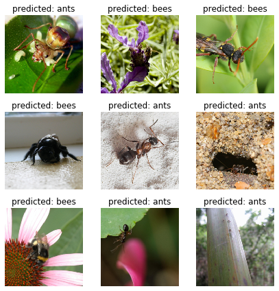
Part 2. Finetuning the Quantizable Model
In this part, we fine tune the feature extractor used for transfer learning, and quantize the feature extractor. Note that in both part 1 and 2, the feature extractor is quantized. The difference is that in part 1, we use a pretrained quantized model. In this part, we create a quantized feature extractor after fine tuning on the data-set of interest, so this is a way to get better accuracy with transfer learning while having the benefits of quantization. Note that in our specific example, the training set is really small (120 images) so the benefits of fine tuning the entire model is not apparent. However, the procedure shown here will improve accuracy for transfer learning with larger datasets.
The pretrained feature extractor must be quantizable. To make sure it is quantizable, perform the following steps:
- Fuse
(Conv, BN, ReLU),(Conv, BN), and(Conv, ReLU)usingtorch.quantization.fuse_modules. - Connect the feature extractor with a custom head. This requires dequantizing the output of the feature extractor.
- Insert fake-quantization modules at appropriate locations in the feature extractor to mimic quantization during training.
For step (1), we use models from torchvision/models/quantization, which have a member method fuse_model. This function fuses all the conv, bn, and relu modules. For custom models, this would require calling the torch.quantization.fuse_modules API with the list of modules to fuse manually.
Step (2) is performed by the create_combined_model function used in the previous section.
Step (3) is achieved by using torch.quantization.prepare_qat, which inserts fake-quantization modules.
As step (4), you can start “finetuning” the model, and after that convert it to a fully quantized version (Step 5).
To convert the fine tuned model into a quantized model you can call the torch.quantization.convert function (in our case only the feature extractor is quantized).
Note: Because of the random initialization your results might differ from the results shown in this tutorial.
# notice `quantize=False`
model = models.resnet18(pretrained=True, progress=True, quantize=False)
num_ftrs = model.fc.in_features

# Step 1
model.train()
model.fuse_model()
# Step 2
model_ft = create_combined_model(model)
model_ft[0].qconfig = torch.quantization.default_qat_qconfig  # Use default QAT configuration
# Step 3
model_ft = torch.quantization.prepare_qat(model_ft, inplace=True)
Finetuning the model
In the current tutorial the whole model is fine tuned. In general, this will lead to higher accuracy. However, due to the small training set used here, we end up overfitting to the training set.
Step 4. Fine tune the model
for param in model_ft.parameters():
  param.requires_grad = True

model_ft.to(device)  # We can fine-tune on GPU if available

criterion = nn.CrossEntropyLoss()

# Note that we are training everything, so the learning rate is lower
# Notice the smaller learning rate
optimizer_ft = optim.SGD(model_ft.parameters(), lr=1e-3, momentum=0.9, weight_decay=0.1)

# Decay LR by a factor of 0.3 every several epochs
exp_lr_scheduler = optim.lr_scheduler.StepLR(optimizer_ft, step_size=5, gamma=0.3)

model_ft_tuned = train_model(model_ft, criterion, optimizer_ft, exp_lr_scheduler,
                              num_epochs=25, device=device)
Epoch 0/24
----------
train Loss: 0.5984 Acc: 0.6762
val Loss: 0.3433 Acc: 0.8758
Epoch 1/24
----------
train Loss: 0.3330 Acc: 0.8525
val Loss: 0.2332 Acc: 0.9216
Epoch 2/24
----------
train Loss: 0.2361 Acc: 0.9180
val Loss: 0.2004 Acc: 0.9346
Epoch 3/24
----------
train Loss: 0.1446 Acc: 0.9590
val Loss: 0.1987 Acc: 0.9281
Epoch 4/24
----------
train Loss: 0.1869 Acc: 0.9385
val Loss: 0.1946 Acc: 0.9216
Epoch 5/24
----------
train Loss: 0.1221 Acc: 0.9713
val Loss: 0.2129 Acc: 0.9216
Epoch 6/24
----------
train Loss: 0.0993 Acc: 0.9672
val Loss: 0.1961 Acc: 0.9281
Epoch 7/24
----------
train Loss: 0.0896 Acc: 0.9754
val Loss: 0.2083 Acc: 0.9281
Epoch 8/24
----------
train Loss: 0.1083 Acc: 0.9672
val Loss: 0.1921 Acc: 0.9412
Epoch 9/24
----------
train Loss: 0.0977 Acc: 0.9672
val Loss: 0.2668 Acc: 0.9020
Epoch 10/24
----------
train Loss: 0.0800 Acc: 0.9877
val Loss: 0.2195 Acc: 0.9085
Epoch 11/24
----------
train Loss: 0.1071 Acc: 0.9631
val Loss: 0.1794 Acc: 0.9412
Epoch 12/24
----------
train Loss: 0.0750 Acc: 0.9672
val Loss: 0.1997 Acc: 0.9216
Epoch 13/24
----------
train Loss: 0.0595 Acc: 0.9877
val Loss: 0.1926 Acc: 0.9281
Epoch 14/24
----------
train Loss: 0.0645 Acc: 0.9877
val Loss: 0.1942 Acc: 0.9281
Epoch 15/24
----------
train Loss: 0.0538 Acc: 0.9836
val Loss: 0.1833 Acc: 0.9346
Epoch 16/24
----------
train Loss: 0.0850 Acc: 0.9754
val Loss: 0.1851 Acc: 0.9412
Epoch 17/24
----------
train Loss: 0.0779 Acc: 0.9754
val Loss: 0.2034 Acc: 0.9216
Epoch 18/24
----------
train Loss: 0.0781 Acc: 0.9713
val Loss: 0.1997 Acc: 0.9150
Epoch 19/24
----------
train Loss: 0.0523 Acc: 0.9918
val Loss: 0.2107 Acc: 0.9150
Epoch 20/24
----------
train Loss: 0.0597 Acc: 0.9836
val Loss: 0.1816 Acc: 0.9281
Epoch 21/24
----------
train Loss: 0.0749 Acc: 0.9754
val Loss: 0.1803 Acc: 0.9346
Epoch 22/24
----------
train Loss: 0.0479 Acc: 0.9959
val Loss: 0.1882 Acc: 0.9346
Epoch 23/24
----------
train Loss: 0.0853 Acc: 0.9631
val Loss: 0.1851 Acc: 0.9346
Epoch 24/24
----------
train Loss: 0.0570 Acc: 0.9918
val Loss: 0.1847 Acc: 0.9281
Training complete in 2m 44s
Best val Acc: 0.941176Step 5. Convert to quantized model
from torch.quantization import convert
model_ft_tuned.cpu()

model_quantized_and_trained = convert(model_ft_tuned, inplace=False)
Lets see how the quantized model performs on a few images
visualize_model(model_quantized_and_trained)

plt.ioff()
plt.tight_layout()
plt.show()