Backpropagation DNN exercises

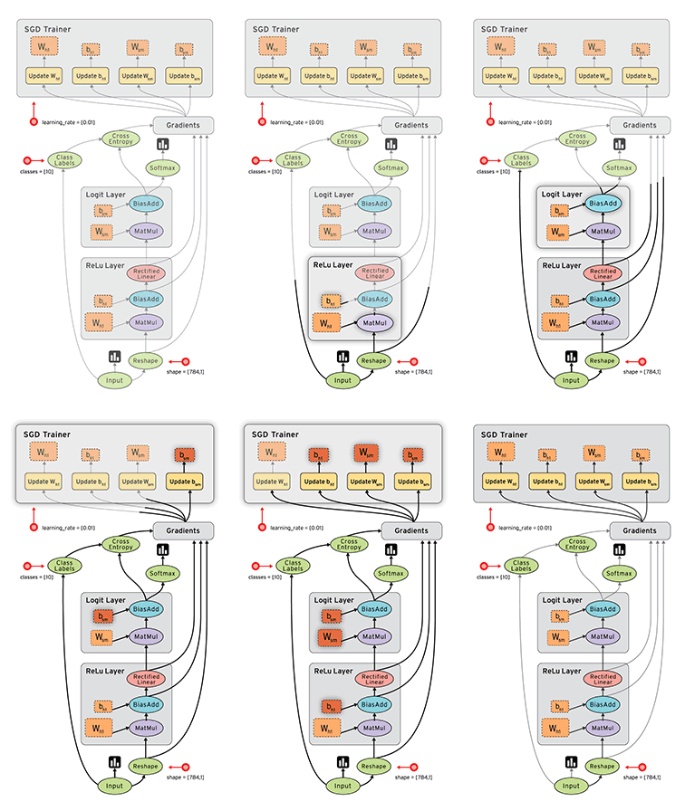
Computational graph in Tensorboard showing the components involved in a TF BP update
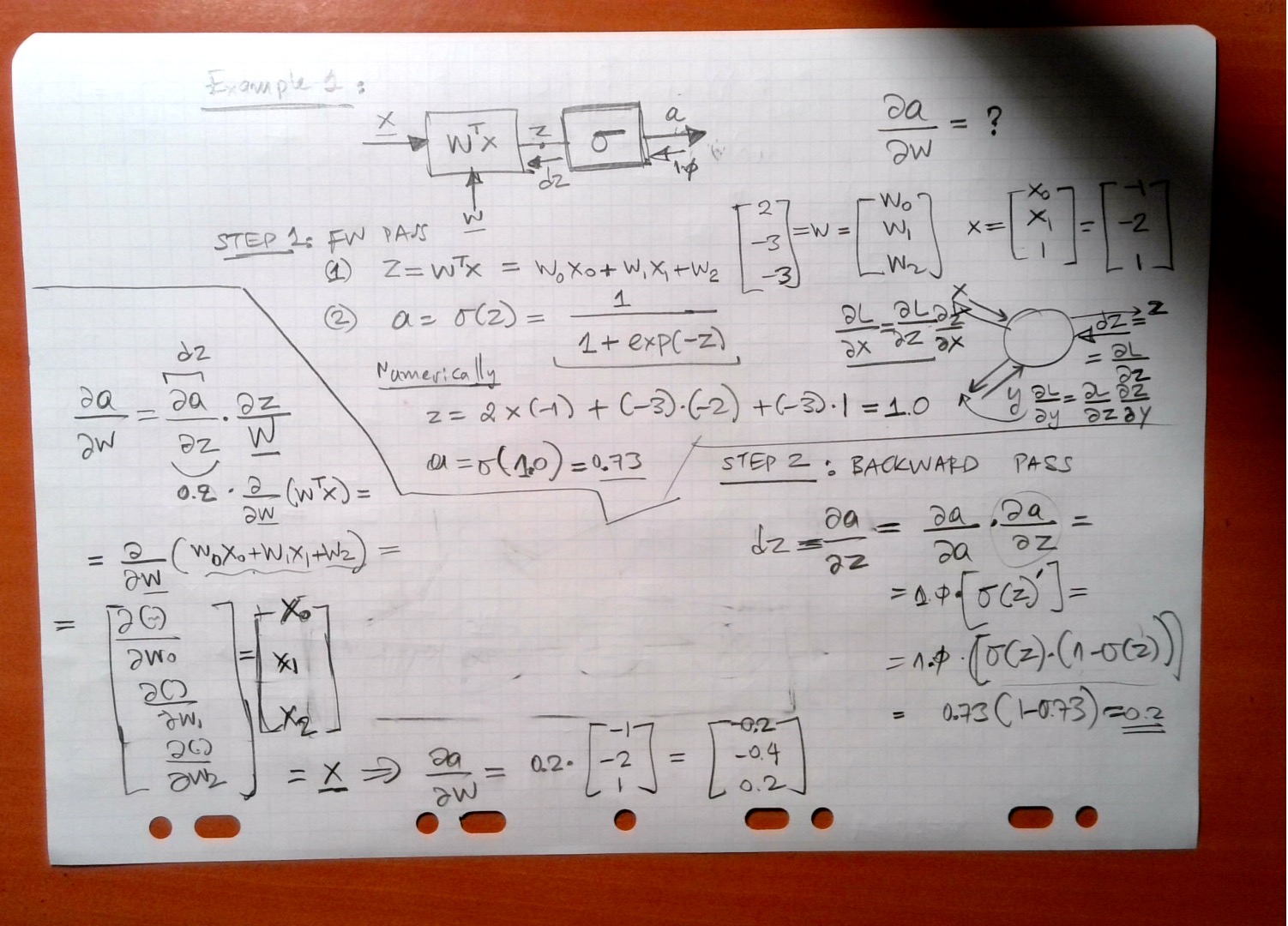
Neuron

Simple DNN 1

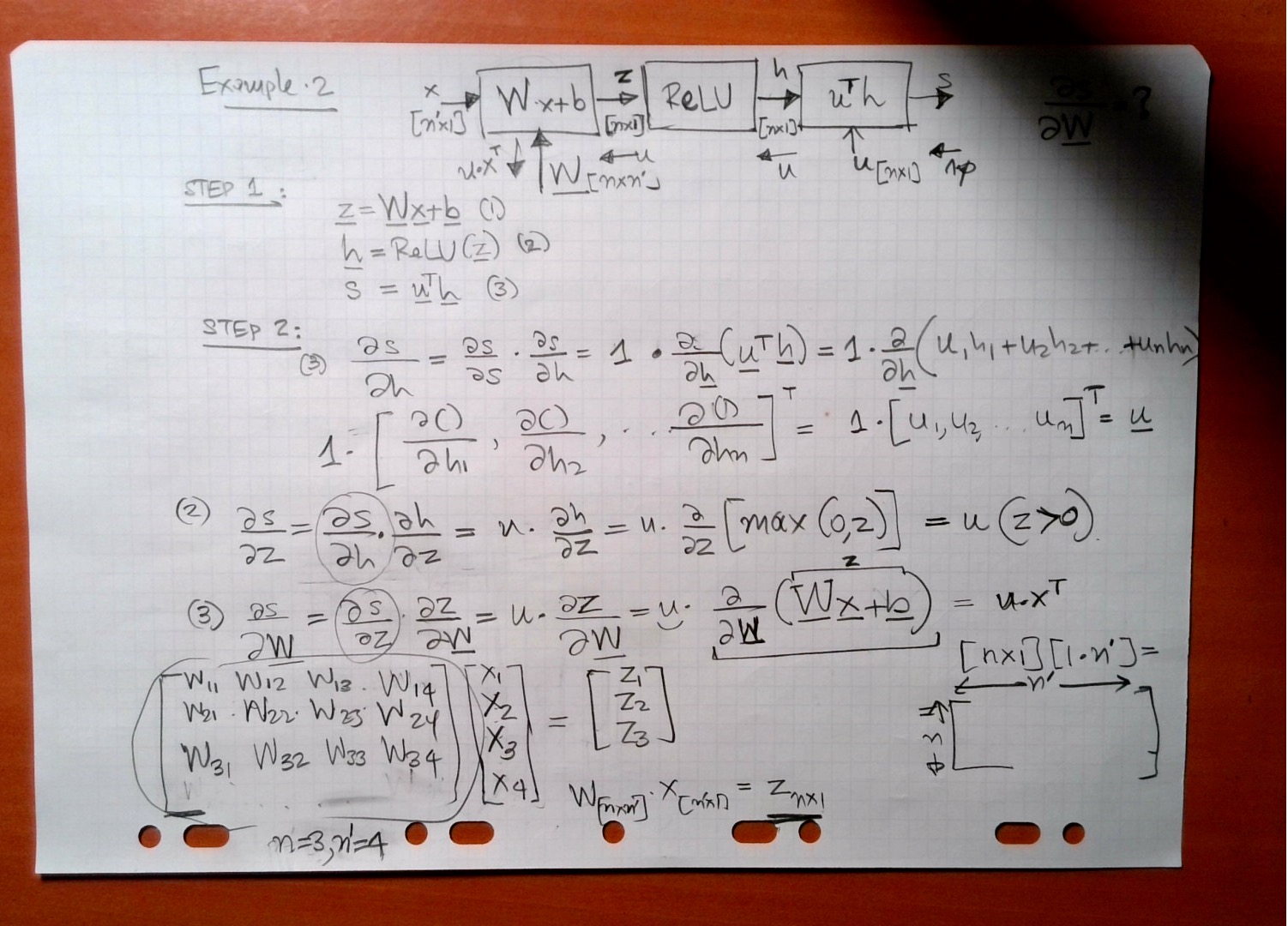
Simple DNN 2
A network consist of a concatenation of the following layers
- Fully Connected layer with input \(x^{(1)}\), \(W^{(1)}\) and output \(z^{(1)}\).
- RELU producing \(a^{(1)}\)
- Fully Connected layer with parameters \(W^{(2)}\) producing \(z^{(2)}\)
- SOFTMAX producing \(\hat{y}\)
- Cross-Entropy (CE) loss producing \(L\)
The task of backprop consists of the following steps:
- Sketch the network and write down the equations for the forward path.
- Propagate the backwards path i.e. make sure you write down the expressions of the gradient of the loss with respect to all the network parameters.
NOTE: Please note that we have omitted the bias terms for simplicity.
| Forward Pass Step | Symbolic Equation |
|---|---|
| (1) | \(z^{(1)} = W^{(1)} x^{(1)}\) |
| (2) | \(a^{(1)} = \max(0, z^{(1)})\) |
| (3) | \(z^{(2)} = W^{(2)} a^{(1)}\) |
| (4) | \(\hat{y} = \mathtt{softmax}(z^{(2)})\) |
| (5) | \(L = CE(y, \hat{y})\) |
| Backward Pass Step | Symbolic Equation |
|---|---|
| (5) | \(\frac{\partial L}{\partial L} = 1.0\) |
| (4) | \(\frac{\partial L}{\partial z^{(2)}} = \hat y - y\) |
| (3a) | \(\frac{\partial L}{\partial W^{(2)}} = a^{(1)} (\hat y - y)\) |
| (3b) | \(\frac{\partial L}{\partial a^{(1)}} = W^{(2)} (\hat y - y)\) |
| (2) | \(\frac{\partial L}{\partial z^{(1)}} = \frac{\partial L}{\partial a^{(1)}}\) if \(a^{(1)} > 0\) |
| (1) | \(\frac{\partial L}{\partial W^{(1)}} = \frac{\partial L}{\partial z^{(1)}} \times x^{(1)}\) |