We have been traditionally normalizing the input data to have a mean of 0 and a standard deviation of 1. This is done to ensure that the input data is centered around 0 and has a similar scale to ensure that the optimization process is stable and converges faster. To see why this helps, consider a limiting example of two parameters as shown below.
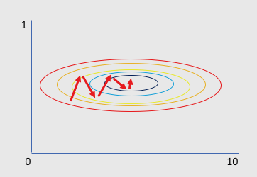
Contour of the loss with respect to two parameters and SGD trajectory
In this contour plot of the loss, the SGD trajectory shown is not smooth which means that the algorithm converges very slowly. As shown in the backpropagation exercise with the single neuron, the gradient of the neuron output with respect to the weight is proportional to the input \(x\) and the proportionality factor can be very small if the dot product is either very large or too small. In the case where all inputs are positive, the changes to the weights are all of the same sign across parameters. The reason is that there is a much larger dynamic range in the x-axis and this means that the gradient with respect to one of the parameters will dominate its direction creating a zig-zag pattern.
The best way to correct the situation is to normalize the input data around a mean of 0 and this will result into a much faster SGD convergence. After normalization you can get a more rounded (bivariate in this case) distribution where gradient directions can be diverse.
Normalizing the input is effective but it is not enough. The reason is that the input data is not the only thing that changes as the data propagates through the network. The distribution of activations also changes which is affected by the value of the parameters (weights).
Parameter initialization
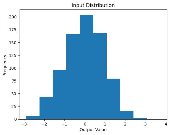
Various techniques have been proposed to address this issue, such as careful initialization of the weights, or using activation functions that are less sensitive to the scale of the weights. In the code below we can see how various initializations can affect the output of a fully connected layer.
import torchimport torch.nn as nnimport torch.optim as optimimport matplotlib.pyplot as pltimport numpy as np# Set up parametersn_input =784n_dense =256# Custom weight and bias initializersclass RandomNormalInitializer:def__init__(self, mean=0.0, std=1.0):self.mean = meanself.std = stddef__call__(self, tensor):return nn.init.normal_(tensor, mean=self.mean, std=self.std)class ZerosInitializer:def__call__(self, tensor):return nn.init.zeros_(tensor)class GlorotNormalInitializer:def__call__(self, tensor):return nn.init.xavier_normal_(tensor)class GlorotUniformInitializer:def__call__(self, tensor):return nn.init.xavier_uniform_(tensor)class HeNormalInitializer:def__call__(self, tensor):return nn.init.kaiming_normal_(tensor, nonlinearity='relu')class HeUniformInitializer:def__call__(self, tensor):return nn.init.kaiming_uniform_(tensor, nonlinearity='relu')# Create a simple MLP modelclass SimpleMLP(nn.Module):def__init__(self, n_input, n_dense, w_init, b_init):super(SimpleMLP, self).__init__()self.fc = nn.Linear(n_input, n_dense)# Initialize weights and biases w_init(self.fc.weight) b_init(self.fc.bias)self.activation = nn.ReLU() #nn.Sigmoid() # You can change to Tanh or ReLU if neededdef forward(self, x): x =self.fc(x) x =self.activation(x)return x# Initialize the modelw_init = HeNormalInitializer() #RandomNormalInitializer(std=1.0) # Replace with desired initializerb_init = ZerosInitializer()model = SimpleMLP(n_input, n_dense, w_init, b_init)# Generate random input valuesx = torch.randn((1, n_input))# Forward propagate through the networka = model(x)x_np = x.detach().numpy() # Convert to numpy for plotting_ = plt.hist(x_np.T)plt.title("Input Distribution")plt.xlabel("Output Value")plt.ylabel("Frequency")plt.show()
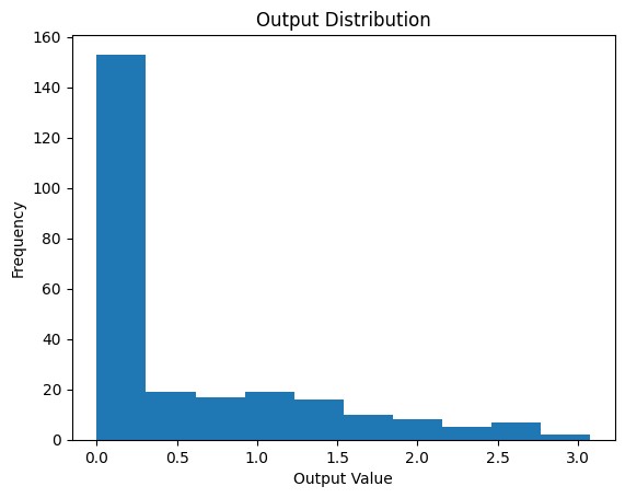
# Plot the outputa_np = a.detach().numpy() # Convert to numpy for plotting_ = plt.hist(a_np.T)plt.title("Output Distribution")plt.xlabel("Output Value")plt.ylabel("Frequency")plt.show()
Bach Normalization
Batch Normalization (Bjorck et al. 2018) alleviates a lot of headaches with properly initializing neural networks by explicitly forcing the activations throughout a network to have a specific distribution during training. Applying this technique amounts to insert the BatchNorm layer immediately after fully connected layers (or convolutional layers), and before activations although empirically we have found that good training behavior is obtained of batch normalization is applied after the activation function (Santurkar et al. 2018). It involves two steps:
Normalization
It normalizes the input to each layer such that the activations have zero mean and unit variance. The key idea here is to explicitly control and stabilize the distribution of the intermediate activations. For each mini-batch during training, the activations are normalized by subtracting the mean and dividing by the standard deviation of the mini-batch. This helps bring the data back to a more consistent distribution with a mean of zero and variance of one.
Where: - \(\mu_{\text{batch}}\) is the mean of the mini-batch.
\(\sigma_{\text{batch}}^2\) is the variance of the mini-batch.
\(\epsilon\) is a small value added to prevent division by zero.
Scaling and Shifting
After normalization, the activations are scaled and shifted using two learnable parameters: \(\gamma\) and \(\beta\). This step allows the network to recover the original representation of the data if necessary and prevents over-restricting the learned features.
\[
y = \gamma \hat{x} + \beta
\]
This scaling and shifting ensure that the transformation is expressive enough to recover any input distribution while keeping it more stable.
The main benefit of Batch Normalization is that of faster convergence, allowing for higher learning rates since it helps to stabilize the training. It also reduces the sensitivity to the initialization of the network parameters.
Intuition of BN
We saw earlier during the treatment of backprop that for a single neuron, the gradient of its output with respect to its parameters is proportional to the input. Extrapolating this observations to a layer of neurons is straightforward. Therefore controlling the statistics of what produced by the previous layer that is input to the current layer is important to ensure that the gradients are just right. We dont know what is just right but we allow the network to let us know by introducing the learnable parameters \(\gamma\) and \(\beta\).
An Example of BN in CNNs
In the provided code, Batch Normalization is implemented manually after each convolutional layer (conv1 and conv2).
During training, the mean and variance are computed based on the mini-batch.
The running mean and variance are updated using a momentum term.
During inference, the running mean and variance are used to normalize the activations instead of the batch statistics since its typical the batch size during training and inference to have different setting.
In practice networks that use Batch Normalization are significantly more robust to parameter initialization. Additionally, batch normalization can be interpreted as doing preprocessing at every layer of the network, but integrated into the network itself in a differentiable manner.
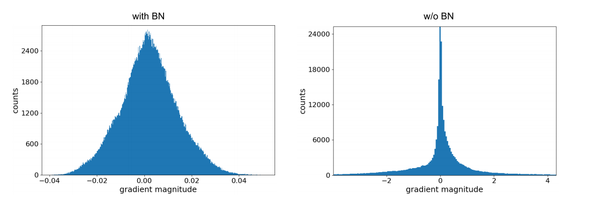
The effects of BN is reflected clearly in the distribution of the gradients for the same set of parameters as shown below.
Histograms over the gradients at initialization for (midpoint) layer 55 of a network with BN (left) and without (right). For the unnormalized network, the gradients are distributed with heavy tails, whereas for the normalized networks the gradients are concentrated around the mean.
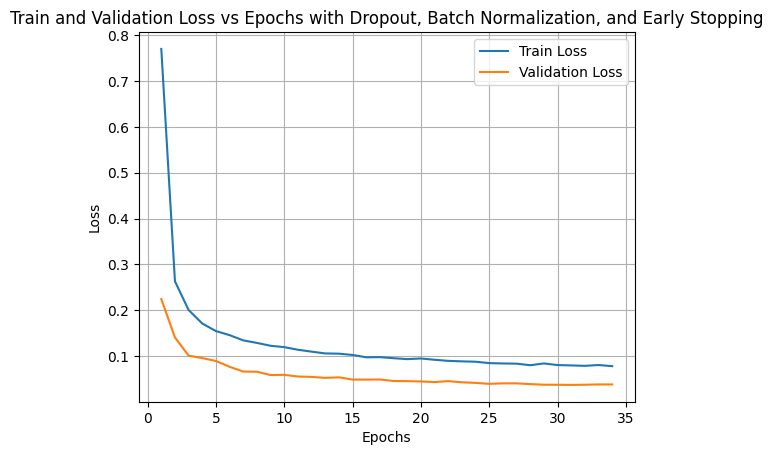
The following code demonstrates the effect of Batch Normalization on a simple neural network.
import torchimport torch.nn as nnimport torch.optim as optimimport torch.nn.functional as Ffrom torchvision import datasets, transformsimport matplotlib.pyplot as pltfrom sklearn.model_selection import train_test_splitimport numpy as npfrom tqdm import tqdm# Define a custom Batch Normalization layerclass CustomBatchNorm(nn.Module):def__init__(self, num_features, eps=1e-5, momentum=0.1):super(CustomBatchNorm, self).__init__()self.num_features = num_featuresself.eps = epsself.momentum = momentumself.gamma = nn.Parameter(torch.ones(num_features))self.beta = nn.Parameter(torch.zeros(num_features))self.running_mean = torch.zeros(num_features)self.running_var = torch.ones(num_features)def forward(self, x):ifself.training:# Calculate batch mean and variance batch_mean = x.mean(dim=[0, 2, 3], keepdim=True) batch_var = x.var(dim=[0, 2, 3], keepdim=True, unbiased=False)# Normalize x_hat = (x - batch_mean) / torch.sqrt(batch_var +self.eps)# Scale and shift out =self.gamma.view(1, -1, 1, 1) * x_hat +self.beta.view(1, -1, 1, 1)# Update running statisticsself.running_mean = (1-self.momentum) *self.running_mean +self.momentum * batch_mean.view(-1)self.running_var = (1-self.momentum) *self.running_var +self.momentum * batch_var.view(-1)else:# Use running mean and variance during inference x_hat = (x -self.running_mean.view(1, -1, 1, 1)) / torch.sqrt(self.running_var.view(1, -1, 1, 1) +self.eps) out =self.gamma.view(1, -1, 1, 1) * x_hat +self.beta.view(1, -1, 1, 1)return out# Define a simple CNN model with custom Batch Normalizationclass SimpleCNN(nn.Module):def__init__(self):super(SimpleCNN, self).__init__()self.conv1 = nn.Conv2d(1, 10, kernel_size=5)self.bn1 = CustomBatchNorm(10)self.conv2 = nn.Conv2d(10, 20, kernel_size=5)self.bn2 = CustomBatchNorm(20)self.fc1 = nn.Linear(320, 50)self.fc2 = nn.Linear(50, 10)self.dropout = nn.Dropout(p=0.5)def forward(self, x): x = F.relu(F.max_pool2d(self.conv1(x), 2)) x =self.bn1(x) x =self.dropout(x) x = F.relu(F.max_pool2d(self.conv2(x), 2)) x =self.bn2(x) x =self.dropout(x) x = x.view(-1, 320) x = F.relu(self.fc1(x)) x =self.fc2(x)return F.log_softmax(x, dim=1)# Set up training parametersbatch_size =64learning_rate =0.01weight_decay =1e-4# L2 regularization parameterpatience =20# Early stopping patience# Load the datasettrain_dataset = datasets.MNIST('../data', train=True, download=True, transform=transforms.ToTensor())train_data, val_data = train_test_split(train_dataset, test_size=0.2, random_state=42)train_loader = torch.utils.data.DataLoader(train_data, batch_size=batch_size, shuffle=True)val_loader = torch.utils.data.DataLoader(val_data, batch_size=batch_size, shuffle=False)# Check if GPU is available and use itdevice = torch.device('cuda'if torch.cuda.is_available() else'cpu')# Initialize the model, loss function, and optimizermodel = SimpleCNN().to(device)criterion = nn.NLLLoss()optimizer = optim.SGD(model.parameters(), lr=learning_rate, weight_decay=weight_decay)# Training loop with Early Stopping and TQDM for Epoch Progressnum_epochs =100train_losses = []val_losses = []min_val_loss = np.infpatience_counter =0for epoch in tqdm(range(num_epochs), desc="Epoch Progress", position=0): model.train() total_train_loss =0for batch_idx, (data, target) inenumerate(train_loader): data, target = data.to(device), target.to(device) optimizer.zero_grad() # Zero the gradients output = model(data) # Forward pass loss = criterion(output, target) # Compute the loss loss.backward() # Backpropagate the gradients optimizer.step() # Update the weights total_train_loss += loss.item() avg_train_loss = total_train_loss /len(train_loader) train_losses.append(avg_train_loss)print(f'Epoch {epoch +1}: Train Loss: {avg_train_loss:.6f}')# Validation loss model.eval() total_val_loss =0with torch.no_grad():for data, target in val_loader: data, target = data.to(device), target.to(device) output = model(data) loss = criterion(output, target) total_val_loss += loss.item() avg_val_loss = total_val_loss /len(val_loader) val_losses.append(avg_val_loss)print(f'Epoch {epoch +1}: Validation Loss: {avg_val_loss:.6f}')# Early stopping checkif avg_val_loss < min_val_loss: min_val_loss = avg_val_loss patience_counter =0 best_model_state = model.state_dict()else: patience_counter +=1if patience_counter >= patience:print(f'Early stopping triggered after {epoch +1} epochs.')break# Load the best model state (if early stopping was triggered)model.load_state_dict(best_model_state)# Plotting Train and Validation Loss vs Epochsplt.plot(range(1, len(train_losses) +1), train_losses, label='Train Loss')plt.plot(range(1, len(val_losses) +1), val_losses, label='Validation Loss')plt.xlabel('Epochs')plt.ylabel('Loss')plt.title('Train and Validation Loss vs Epochs with Dropout, Batch Normalization, and Early Stopping')plt.legend()plt.grid(True)plt.show()
/usr/local/lib/python3.10/dist-packages/torch/cuda/__init__.py:128: UserWarning: CUDA initialization: CUDA unknown error - this may be due to an incorrectly set up environment, e.g. changing env variable CUDA_VISIBLE_DEVICES after program start. Setting the available devices to be zero. (Triggered internally at ../c10/cuda/CUDAFunctions.cpp:108.)
  return torch._C._cuda_getDeviceCount() > 0
Epoch Progress:   0%|          | 0/50 [00:00<?, ?it/s]
Epoch 34: Train Loss: 0.077929
Epoch 34: Validation Loss: 0.038055
Early stopping triggered after 34 epochs.
References
Bjorck, Nils, Carla P Gomes, Bart Selman, and Kilian Q Weinberger. 2018. “Understanding Batch Normalization.” In Advances in Neural Information Processing Systems 31, edited by S Bengio, H Wallach, H Larochelle, K Grauman, N Cesa-Bianchi, and R Garnett, 7694–7705. Curran Associates, Inc.
Santurkar, Shibani, Dimitris Tsipras, Andrew Ilyas, and Aleksander Madry. 2018. “How Does Batch Normalization Help Optimization?”arXiv [Stat.ML], May.