Deep Neural Networks

DNNs are the implementation of connectionism, the philosophy that calls for algorithms that perform function approximations to be constructed by an interconnection of elementary circuits called neurons. In this section, we provides some key points on the question of how the feed-forward neural networks are constructed. In subsequent sections we describe how they learn.

Architecture

Feedforward networks consist of elementary units that resemble the logistic regression architecture. Multiple units form a layer and there are multiple layers types:

1. The input layer
2. One or more hidden layers (also known as the body)
3. The output layer (also known as the head)

Since the input to the network is trivial we focus on the hidden and output layers starting from the latter.

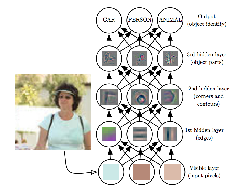Example DNN Architecture emphasizing the hierarchical build up of more complex features.

Output Layer

The feedforward network provides a set of hidden features defined by

$$\mathbf{h}=f(\mathbf{x};\mathbf{w})$$

The role of the output layer is then to provide some additional transformation from the features to complete the task that the network must perform.

Sigmoid Units

These are used to predict the value of the binary variable $y$. As evident in logistic regression, using a sigmoid output units combined with maximum likelihood provides a very strong response when we are confidently wrong. A sigmoid output unit is defined by

$$\mathbf{z}={\mathbf{w}}^T\mathbf{h}+b$$ $$\hat{y}=\sigma (\mathbf{z})$$

where the sigmoid activation function

$$g(a)=\sigma (a)=\frac{1}{1+e^{-a}}\sigma (a)\in (0,1)$$

Towards either end of the sigmoid function, the $\sigma (a)$ values tend to respond much less to changes in a vanishing gradients. The neuron refuses to learn further or learns drastically slower that it could. What saves the situation is the log loss that undoes the exp of the sigmoid but this is the case for the final layers -this is the reason why normalization is usually used in each layer.

Softmax Units

Any time we wish to represent a probability distribution over a discrete variable with $n$ possible values, we may use the softmax function. This can be seen as a generalization of the sigmoid function, which was used to represent a probability distribution over a binary variable. Softmax functions are most often used as the output of a classifier, to represent the probability distribution over $n$ different classes. The softmax output unit is effectively a generalization of the sigmoid.

$$\text{softmax}(\mathbf{z}{)}_i=\arg \underset{i}{max}\frac{\exp (z_i)}{\sum _i\exp (z_i)}$$

where $i$ is over the number of inputs of the softmax function.

From a neuroscientific point of view, it is interesting to think of the softmax as a way to create a form of competition between the units that participate in it: the softmax outputs always sum to 1 so an increase in the value of one unit necessarily corresponds to a decrease in the value of others. This is analogous to the lateral inhibition that is believed to exist between nearby neurons in the cortex. At the extreme (when the difference between the maximal and the others is large in magnitude) it becomes a form of winner-take-all(one of the outputs is nearly 1, and the others are nearly 0).

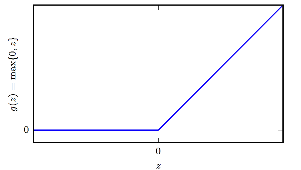
ReLUs

The Rectified Linear Unit activation function is very inexpensive to compute compared to sigmoid and it offers the following benefit that has to do with sparsity: Imagine an MLP with random initialized weights to zero mean ( or normalized ). Almost 50% of the network yields 0 activation because of the characteristic of RELU. This means a fewer neurons are firing (sparse activation) making the the network lighter, more efficient that tends to generalize to validation data better. On the other hand for negative $a$, the gradient can go towards 0 and the weights will not get adjusted during descent. As a testament to its utility, the incorporation of ReLU neurons into AlexNet was one of the factors behind its trampling of existing machine vision benchmarks in 2012 and shepherding in the era of deep learning. Since then more advanced activation functions have been proposed such as the leaky ReLU, the parametric ReLU, and the exponential linear unit—all three of which are derivations from the ReLU neuron.

relu

Cross Entropy (CE) Loss

This is used for multiclass classification problems.

It offers certain advantages during the learning of deep neural networks. Given that the gradient must be large enough to act as a guiding direction during SGD, we need to avoid situations that the output units result in flat responses (saturate). Since softmax involves exponentials, it saturates when for example the differences between inputs become extreme. The CE loss helps as the log undoes the exponential terms.

Putting it all together

Tensorflow and Pytorch can log the computational graph associated with a DNN model allowing you to visualize it using Tensorboard. Use the playground when you first learn about DNNs to understand the principles regarding increasing the complexity of the hypothesis by connecting multiple neurons together but dive into the Fashion MNIST use case to understand the mechanics and how to debug models python scripts both syntactically and logically. Logical debugging involves logging and plotting the loss functions and other metrics (for classification this may be for example per-class accuracy).

Other resources

For a historical recap on neural networks see:

The Epistemology of Deep Learning - Yann LeCun

For an astonishing visualization of the learning process of a (dense) neural network see:

But what is a neural network?