Cameras and Image Processing
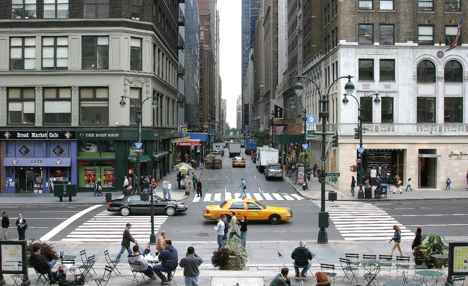
As elaborated here, humans build up a more schematic version of the environment across eye fixations than was previously thought. This schematic version of the environment is typically known as scene gist. It contains conceptual information about the scene’s basic category – is it natural, human-made, a cityscape perhaps – and general layout, maybe limited to a few objects and/or features. This schematic version of the environment is a far cry from the “picture in the head” scenario. But it’s this schematic information that guides us from one eye fixation to the next, during which more detailed information can be sampled. In the picture above, the brain will first detect the cityscape schematic and then process one of the scene fixations - e.g. the yellow cab.
Neuroscientists David Hubel and Torsten Wiesel defined the so called V1 region of the brain - the region at the back of our head that is responsible for the processing of visual sensory input signals coming from the eye’s retina and researchers modelled this region as stacks of convolutional neural layers. Before going into the details of such layers, we will first look at the cameras sensors and how they capture images. Futher since no sensor is ideal, we will also look at camera calibration that is used to account for such imperfections and improve the quality of the captured images and by extension the quality of the geometric information that we can extract from them.
Color images as functions
We typically refer to the size of the image as \(w \times h\) where \(w\) is the width (number of columns) and \(h\) is the height (number of rows). We write the image as a tensor, a matrix in this grayscale case, \(\mathbf x(i,j)\) where the convention is to refer to the columns \(j\) of the matrix that represents each function with \(x\) and to the rows \(i\) with \(y\) - this may cause some confusion at first.
A function \(f(i,j)\) maps the pixel coordinates to the intensity value at that pixel. The dynamic range of intensity values depend on how many bits the sensor has been manufactured with. Typically we see 8-bits per pixel therefore limiting the dynamic range to [0, 255], although some cameras can capture images with 10, 12 or even 16 bits per pixel.
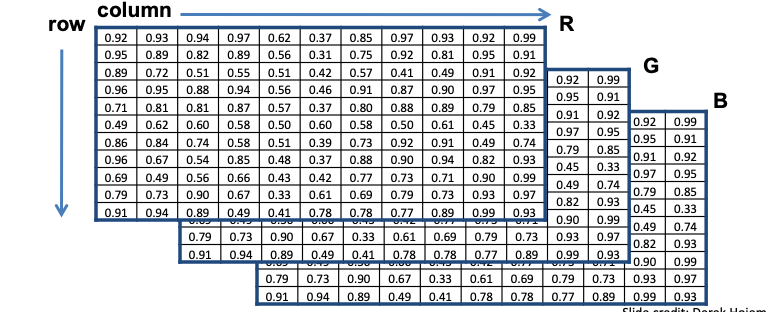
Most of the real world is however, captured in color. The naturally colored image in Figure 1 can be seen as a vector function:
\[\mathbf f(i,j)= \begin{bmatrix} r(i,j) \\ g(i,j) \\ b(i,j) \end{bmatrix}\]
with the 3rd dimension assigned to the image channels. If these corresponds to the well known Red, Green and Blue fundamental colors, we call this the RGB color space encoding. The mixture or superposition of these channels can generate each pixel color of the original image.
Image Normalization
Before processing images we need to convert them to floating point values in the range [0, 1]. This is called normalization and it is done by dividing each pixel value by the maximum value of the channel. For example, if we have an RGB image with pixel values in the range [0, 255], we normalize it as follows:
\[\mathbf x_{norm}(i,j) = \begin{bmatrix} \frac{r(i,j)}{255} \\ \frac{g(i,j)}{255} \\ \frac{b(i,j)}{255} \end{bmatrix}\]