Beam-based sensor models

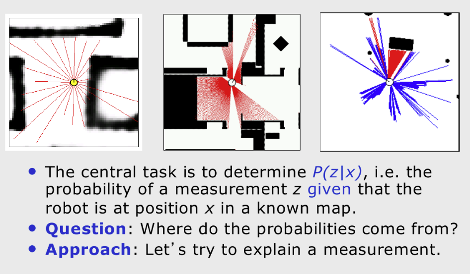
Beam-based distance sensors (sonar, lidar, depth IR) measure distances to the nearest surface along discrete directions (beams). We develop a probabilistic forward (generative) model \(p(\mathbf z_t \mid \mathbf x_t, m)\) describing the likelihood of receiving range scan \(\mathbf z_t\) from pose \(\mathbf x_t\) in map \(m\), and an inverse model for occupancy mapping.
Notation:
- Robot pose (planar): \(\mathbf x_t = (x_t, y_t, \theta_t)\).
- Map \(m\): occupancy grid (binary / probabilistic) or geometric (polygonal, mesh).
- Scan: \(\mathbf z_t = \{ z_t^k \}_{k=1}^K\) with beam angles \(\phi_k\) relative to sensor frame.
- Maximum sensor range: \(z_{\max}\).
- Expected (ideal) range along beam \(k\): \(\hat z_t^k = r(\mathbf x_t, \phi_k, m)\) found via ray casting.
Assumed conditional independence (approximation): \[ p(\mathbf z_t \mid \mathbf x_t, m) = \prod_{k=1}^K p(z_t^k \mid \mathbf x_t, m). \]

Beam-Based Forward Model (Mixture)
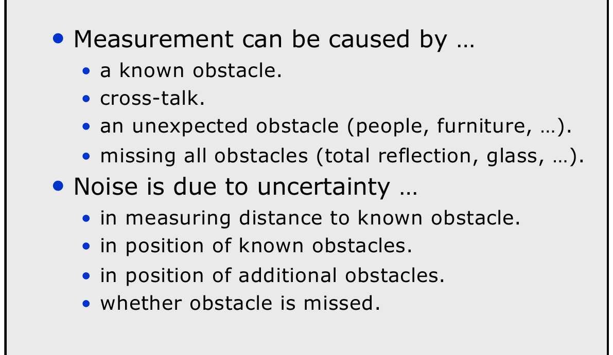
Real measurements exhibit multiple phenomena: precise hits, unexpected short returns, max-range (no return), and random noise. Model each beam as a weighted mixture: \[ p(z \mid \hat z) = \alpha_{\text{hit}} p_{\text{hit}}(z \mid \hat z) + \alpha_{\text{short}} p_{\text{short}}(z \mid \hat z) + \alpha_{\text{max}} p_{\text{max}}(z) + \alpha_{\text{rand}} p_{\text{rand}}(z), \] with \(\sum_i \alpha_i = 1\).
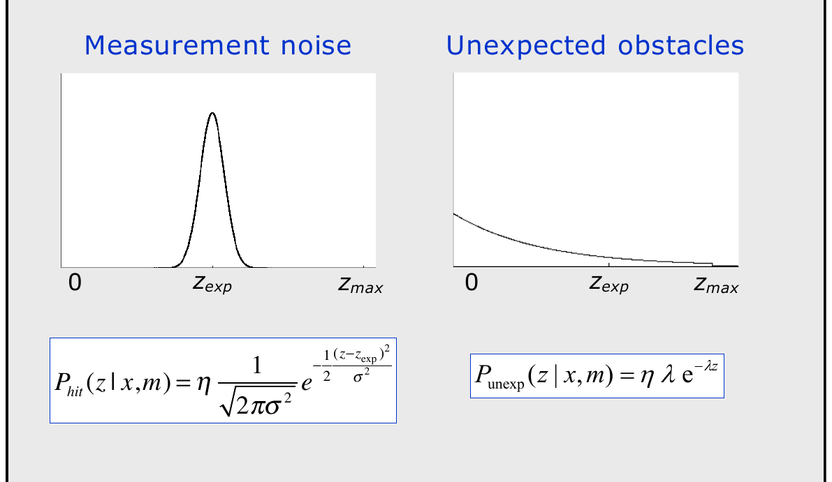
 {fig-hit-unexpected-components}
Precise Hit Component
\[ p_{\text{hit}}(z \mid \hat z) = \begin{cases} \eta \exp\!\left(-\dfrac{(z - \hat z)^2}{2\sigma_{\text{hit}}^2}\right), & 0 \le z \le z_{\max}\\ 0, & \text{otherwise} \end{cases} \] \(\eta\) normalizes over \([0,z_{\max}]\).
Unexpected Short Return
Captures unmodelled obstacles between sensor and predicted surface: \[ p_{\text{short}}(z \mid \hat z) = \begin{cases} \eta \lambda e^{-\lambda z}, & 0 \le z \le \hat z\\ 0, & z > \hat z \end{cases} \]
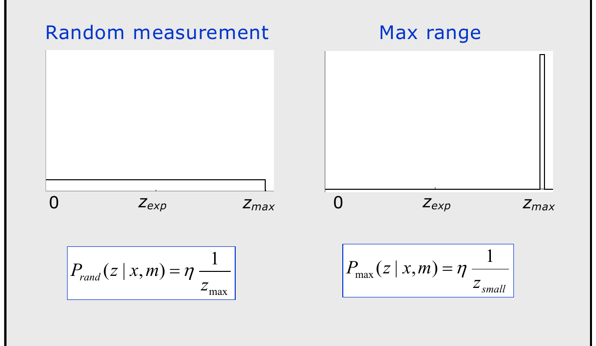
 {fig-random-max-range-components}
Max Range
\[ p_{\text{max}}(z) = \begin{cases} 1, & z = z_{\max}\\ 0, & \text{otherwise} \end{cases} \]
Random Noise
\[ p_{\text{rand}}(z) = \begin{cases} \dfrac{1}{z_{\max}}, & 0 \le z < z_{\max}\\ 0, & \text{otherwise} \end{cases} \]
Final Per-Beam Likelihood
\[ p(z_t^k \mid \mathbf x_t, m) = p(z \mid \hat z_t^k). \]
Log form for numerical stability: \[ \log p(\mathbf z_t \mid \mathbf x_t, m) = \sum_k \log\left( \sum_j \alpha_j p_j(z_t^k) \right). \]
Parameter Estimation
Given training set \(\{ (z_n, \hat z_n)\}\):
- Closed-form for \(\sigma_{\text{hit}}^2\) using weighted residual variance if component assignments known.
- Use EM:
- E-step: responsibilities \(r_{ni} = \dfrac{\alpha_i p_i(z_n)}{\sum_j \alpha_j p_j(z_n)}\).
- M-step: \(\alpha_i = \frac{1}{N}\sum_n r_{ni}\); update \(\sigma_{\text{hit}}, \lambda\) via weighted MLE.
Constrain \(\alpha_i \ge 0\), \(\sum\alpha_i=1\).
Dynamic Obstacles
Augment forward model with dynamic layer \(m_D\): \[ p(z \mid \hat z, m, m_D) = (1-\beta) p(z \mid \hat z, m) + \beta p_{\text{dyn}}(z), \] where \(p_{\text{dyn}}\) could emphasize short / random returns; \(\beta\) from motion segmentation.