Online Prediction
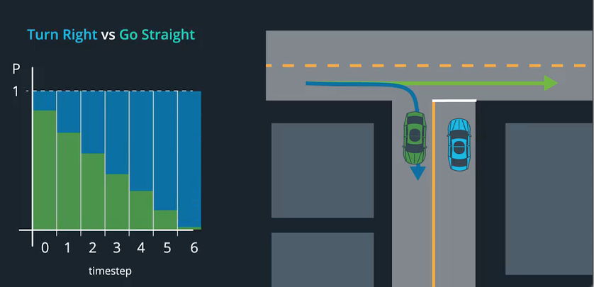
To understand the motion prediction subsystem, we can use an example. Our agent arrives in an T-shaped intersection and perceives that there is another agent approaches from the left. The other agent may be doing two things:
- Slowing down and turning right into the road that our agent is on.
- Going straight.
Via the perception subsystem our agent the moment it predicts that the other agent is slowing down (indicating perhaps also its intention to turn right), it can start turning left long before the other agent’s manuever is completed, improving its efficiency / utility - after all the average speed may be one of the desirable metrics.
Thinking probabilistically, we need to maintain a belief, regarding the location of the turning-right agent. This belief will change over time as its updated with new observations.
Model vs Data-driven approaches to prediction
Already we have used offline maps that provide the static world that the agent operates in to do route planning. Such maps are constructed automatically from aerial imaging and information from the agent’s perception systems is used to simultaneously localize the ego agent and map its surroundings (a function called SLAM). In this section we continue to assume that such maps exists and we now need to determine how we capture the presence of dynamic objects on such maps.
We assume that the sensing and perception subsystems provide the following information for each dynamic object (other agent).
\[[id, x, y, v_x, v_y, \sigma_x, \sigma_y, \sigma_{vx} \sigma_{vy}]^T\]
The prediction output will be a list of trajectories each specified by a list of \([x, y, \mathtt{yaw}, \mathtt{timestamp}]\) elements and tagged with a probability. Each trajectory has a horizon of few (e.g. 10s) seconds and typically their time resolution is 200ms.
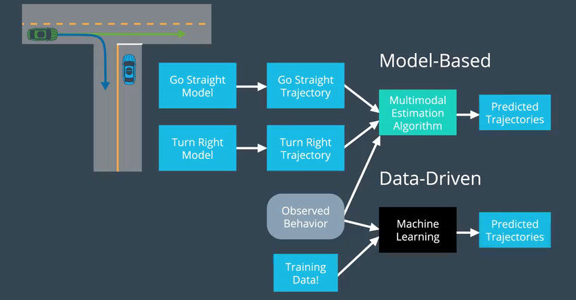
To estimate the probabilities of the possible trajectories we have two broad options:
Model-based approach. In this approach, we use process models to generate trajectories for each of the possible hypotheses we have. The models capture the dynamics of each agent, the rules governing how an agent must turn etc. We use the perception subsystem and an estimation algorithm to estimate the belief (posterior) that the other agent will follow each of the reference trajectories.
ML-based approach. In this approach, the probabilities are estimated using supervised learning methods where we need to label the observations according to the trajectory that the agent followed. We use such training data to train a model that will predict the class (trajectory ID) and the confidence (belief).