Value Iteration
We already have seen that in the Gridworld example in the policy iteration section , we may not need to reach the optimal state value function \(v_*(s)\) to obtain an optimal policy result. The value function for the \(k=3\) iteration results the same policy as the policy from a far more accurate value function (large k).
We could have stopped early and taking the argument to the limit, we can question the need to start from a policy altogether. Instead of letting the policy \(\pi\) dictate which actions are selected, we will select those actions that maximize the expected reward. We therefore do the improvement step in each iteration computing the optimal value function without a policy.
In this section we will look at an algorithm called value iteration that does that.
The basic principle behind value-iteration is the principle that underlines dynamic programming and is called the principle of optimality as applied to policies. According to this principle an optimal policy can be divided into two components.
An optimal first action \(a_*\).
An optimal policy from the successor state \(s^\prime\).
More formally, a policy \(\pi(a|s)\) achieves the optimal value from state \(s\), \(v_\pi(s) = v_*(s)\) iff for any state \(s^\prime\) reachable from \(s\), \(v_\pi(s^\prime)=v_*(s)\).
Effectively this principle allows us to decompose the problem into two sub-problems with one of them being straightforward to determine and use the Bellman optimality equation that provides the one step backup induction at each iteration.
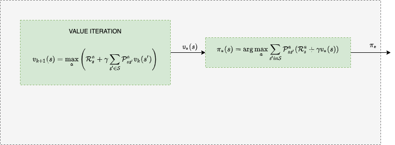
\[v_*(s) = \max_a \left( \mathcal R_s^a + \gamma \sum_{s^\prime \in \mathcal S} \mathcal{P}^a_{ss^\prime} v_*(s^\prime) \right)\]
As an example if I want to move optimally towards a location in the room, I can make a optimal first step and at that point I can follow the optimal policy, that I was magically given, towards the desired final location. That optimal first step, think about making it by walking backwards from the goal state. We start at the end of the problem where we know the final rewards and work backwards to all the states that connect to it in our look-ahead tree.
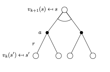
The “start from the end” intuition behind the equation is usually applied with no consideration as to if we are at the end or not. We just do the backup inductive step for each state. In value iteration for synchronous backups, we start at \(k=0\) from the value function \(v_0(s)=0.0\) and at each iteration \(k+1\) for all states \(s \in \mathcal{S}\) we update the \(v_{k+1}(s)\) from \(v_k(s)\). As the iterations progress, the value function will converge to \(v_*\).
The equation of value iteration is taken straight out of the Bellman optimality equation, by turning the later into an update rule called the Bellman update.
\[v_{k+1}(s) = \max_a \left( \mathcal R_s^a + \gamma \sum_{s^\prime \in \mathcal S} \mathcal{P}^a_{ss^\prime} v_k(s^\prime) \right) \]
The value iteration can be written in a vector form as,
\[\mathbf v_{k+1} = \max_a \left( \mathcal R^a + \gamma \mathcal P^a \mathbf v_k \right) \]
Notice that we are not building an explicit policy at every iteration and also, importantly, the intermediate value functions may not correspond to a feasible policy.
Value Iteration in Gridworld Example
Some of the figures quote utility - this is synonymous to value
To solve the non-linear equations for \(v^{*}(s)\) we use an iterative approach.
Steps:
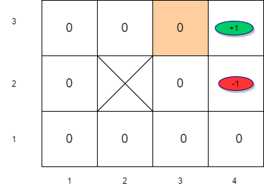
Initialize estimates for the utilities of states with arbitrary values: \(v(s) \leftarrow 0 \forall s \epsilon S\)
Next use the iteration step below repeatedly. Since we are taking \(\max\) we only need to consider states whose next states have a positive value.
\[v_{k+1}(s) \leftarrow R(s) + \gamma \underset{a}{ \max} \left[ \sum_{s^{'}} P(s^{'}| s,a) v_k(s^{'}) \right] \forall s \epsilon S\]
- Let us apply this to the maze example. Assume that \(\gamma = 1\) for simplicity.
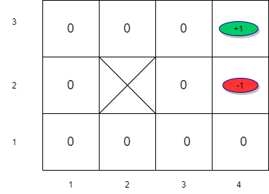
- For the remaining states, the value is equal to the immediate reward in the first iteration.
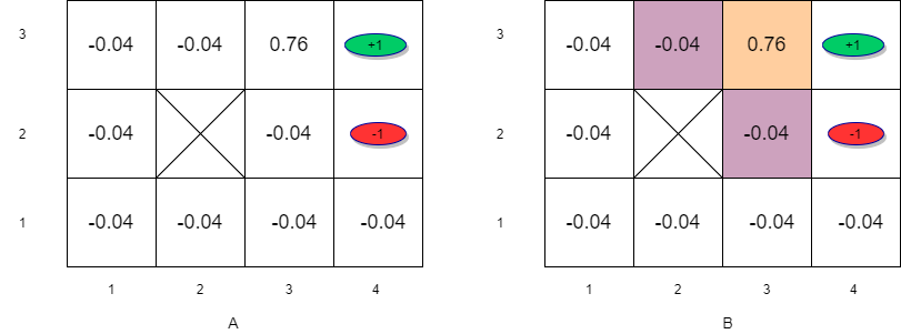
Value Iteration (k=1)
\[v_1(s_{33}) = R(s_{33}) + \gamma \max_a \left[\sum_{s^{'}} P(s^\prime| s_{33},a)v(s{'}) \right] \forall s \in S \]
\[v_1(s_{33}) = -0.04 + \max_a \left[ \sum_{s'} P(s'| s_{33},\uparrow) v_0(s'), \sum_{s'} P(s'| s_{33},\downarrow)v_0(s'), \sum_{s'} P(s'| s_{33},\rightarrow) v_0(s'), \sum_{s'} P(s'| s_{33}, \leftarrow)v_0(s') \right]\]
\[v_1(s_{33}) = -0.04 + \sum_{s^{'}} P(s^{'}| s_{33},\rightarrow) v_0(s^\prime) \]
\[v_1(s_{33}) = -0.04 + P(s_{43}|s_{33},\rightarrow)v(s_{43})+P(s_{33}|s_{33},\rightarrow)v(s_{33})+P(s_{32}|s_{33},\rightarrow)v_0(s_{32}) \]
\[v_1(s_{33}) = -0.04 + 0.8 \times 1 + 0.1 \times 0 + 0.1 \times 0 = 0.76 \]
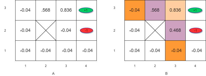
Value Iteration (k=2)
\[v_2(s_{33}) = -0.04 + P(s_{43}|s_{33},\rightarrow)v_1(s_{43})+P(s_{33}|s_{33},\rightarrow)v_1(s_{33}) +P(s_{32}|s_{33},\rightarrow)v_1(s_{32}) \]
\[v_2(s_{33}) = -0.04 + 0.8 \times 1 + 0.1 \times 0.76 + 0.1 \times 0 = 0.836\]
\[v_2(s_{23}) = -0.04 + P(s_{33}|s_{23},\rightarrow)v_1(s_{23})+P(s_{23}|s_{23},\rightarrow)v_1(s_{23}) = -0.04 + 0.8 \times 0.76 = 0.568\]
\[v_2(s_{32}) = -0.04 + P(s_{33}|s_{32},\uparrow)v_1(s_{33})+P(s_{42}|s_{32},\uparrow)v_1(s_{42}) +P(s_{32}|s_{32},\uparrow)v_1(s_{32})\] \[v_2(s_{32}) = -0.04 + 0.8 \times 0.76 + 0.1 \times -1 + 0.1 \times 0= 0.468\]
Value Iteration (k=3)
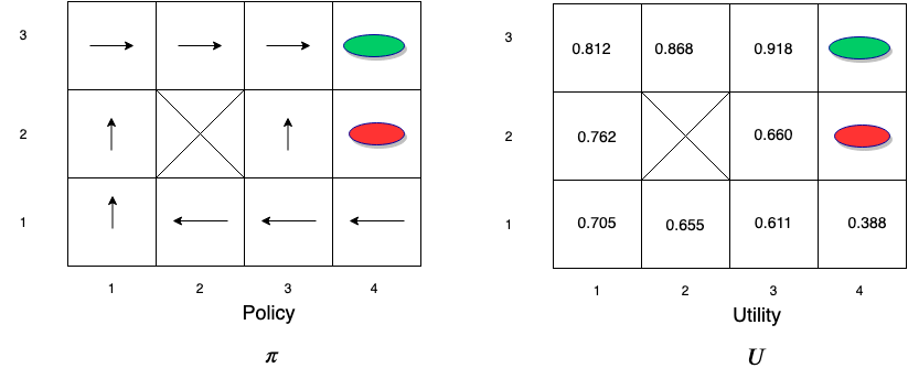
Notice how information propagates outward from terminal states and eventually all states have correct value estimates. \(s_{32}\) has a lower value compared to \(s_{23}\) due to the red oval state with negative reward next to \(s_{32}\)
After many iterations, the value estimates converge to the optimal value function \(v^*(s)\) and a policy \(\pi^*\) can be derived from the value function using the following equation:
\[\pi^*(s) = \arg \max_a \left[ \sum_{s^{'}} P(s^{'}| s,a)v^*(s^{'}) \right]\]
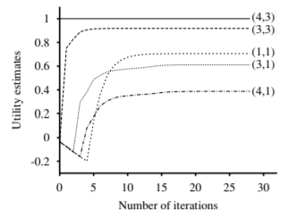
Value Iteration - Convergence
The rate of convergence depends on the maximum reward value and more importantly on the discount factor \(\gamma\). The policy that we get from coarse estimates is close to the optimal policy long before \(v\) has converged. This means that after a reasonable number of iterations, we could extract the policy in a greedy fashion and use it to guide the agent’s actions.