The SARSA Algorithm
SARSA implements a \(Q(s,a)\) value-based GPI and naturally follows as an enhancement from the \(\epsilon-greedy\) policy improvement step of MC control.
We meet also here the familiar two steps:
The first is a technique for learning the Q-function via TD-learning that we have seen in the prediction section.
The second is a method for evolving the policy using the learned Q-function.
SARSA - TD Learning
In the TD prediction section, we have met the TD prediction step for \(V(s)\) but for control we need to predict the \(Q(s,a)\).
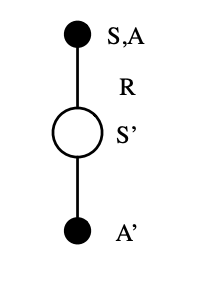
The TD(0), also known as single-step TD, tree for SARSA is shown below:

SARSA action-value backup update tree. Its name is attributed to the fact that we need to know the State-Action-Reward-State-Action before performing an update.
Following the value estimate of temporal difference (TD) learning, we can write the value update equation as:
\[Q(S,A) = Q(S,A) + \alpha (R + \gamma Q(S^\prime, A^\prime)-Q(S,A))\]
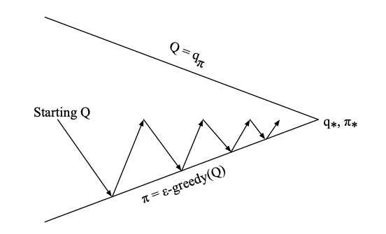
Effectively the equation above updates the Q function by \(\alpha\) times the direction of the TD error. What SARSA does is basically the policy iteration diagram we have seen in the control above but with a twist. Instead of trying to evaluate the policy using episodes as in MC, SARSA does policy improvement on an estimate obtained over each time step significantly increasing the iteration rate - this is figuratively shown below:

SARSA on-policy control
The idea is to increase the frequency of the so called \(\epsilon\)-greedy policy improvement step where we select with probability \(\epsilon\) a random action instead of the action that maximizes the \(Q(s,a)\) function (greedy). We do so, in order to “hit” new states and therefore improve on the degree of exploration of our agent and as a result giving opportunities to the agent to reduce its variance and its bias.
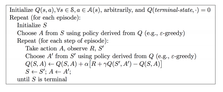
The SARSA algorithm is summarized below:

SARSA algorithm for on-policy control