Contrastive Language-Image Pretraining (CLIP)
Language is a representation of our world and so is perception - both language and vision are trying to solve the same problem.
We saw in ?@sec-word2vec that a prediction task can be used to learn a representation of a word - recall we are predicting the words that are frequent closeby. This type of task is called a pretext task. The idea is that if we learn a prediction task that dependents on a representation and our predictions are correct, then we have learned a good representation.
This is a very general idea and it applies to many different domains. For example, in vision, we can use a pretext task to learn a representation of an image by predicting the pixels in the image. This is called self-supervised learning because we are using the data itself to supervise the learning process.
Self-supervised Learning
In NLP labeled data for representation learning are plentiful but in computer vision they are quite scarce. When we don’t have labeled targets we try to create virtual targets out of the raw data itself. This idea is called self-supervision. It looks like this:
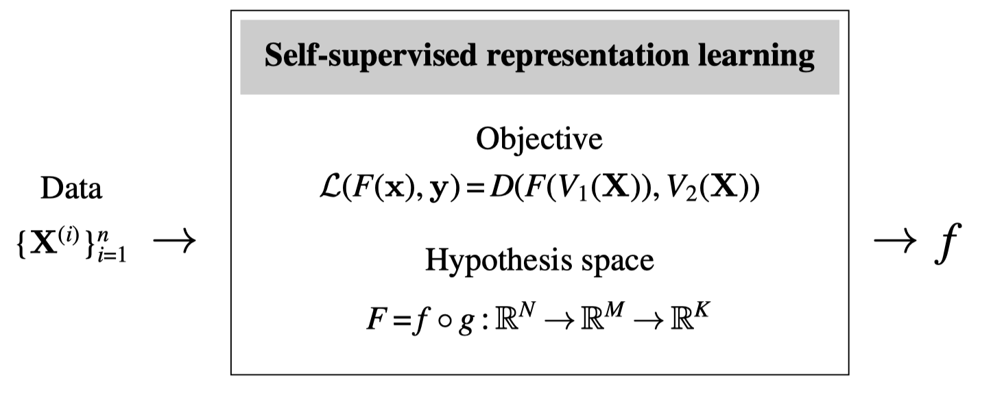
where \(V_1\) and \(V_2\) are two different functions of the full data tensor \(\mathbf{X}\). For example, \(V_1\) might be the left side of the image \(\mathbf{X}\) and \(V_2\) could be the right side, so the pretext task is to predict the right side of an image from its left side. In fact, several of the examples we gave previously for predictive learning are of the self-supervised variety: supervision for predicting a future frame, or a next pixel, can be cooked up just by splitting a video into past and future frames, or splitting an image into previous and next pixels in a raster-order sequence.
Contrastive Learning
Dimensionality reduction and clustering algorithms learn compressed representations by creating an information bottleneck, that is, by constraining the number of bits available in the representation. An alternative compression strategy is to supervise what information should be thrown away. Contrastive learning is one such approach where a representation is supervised to be invariant to certain viewing transformations, resulting in a compressed representation that only captures the properties that are common between the different data views. Two different data views could correspond to two different cameras looking at the same scene or two different imaging modalities, such as color and depth, and we will see more examples subsequently.
Contrastive learning is actually more closely related to clustering than it may at first seem. Contrastive learning maps similar datapoints to similar embeddings. Clustering is just the extreme version of this where there are only \(k\) distinct embeddings and similar datapoints get mapped to the exact same embedding.
Learning invariant representations is classic goal of computer vision. Recall that this was one of the reasons we used convolutional image filters: convolution is equivariant with camera translation, and invariance can then be achieved simply by pooling over filter responses. CNNs, through their convolutional architecture, bake translation invariance into the hypothesis space. In this section we will see how to incentivize invariances instead through the objective function.
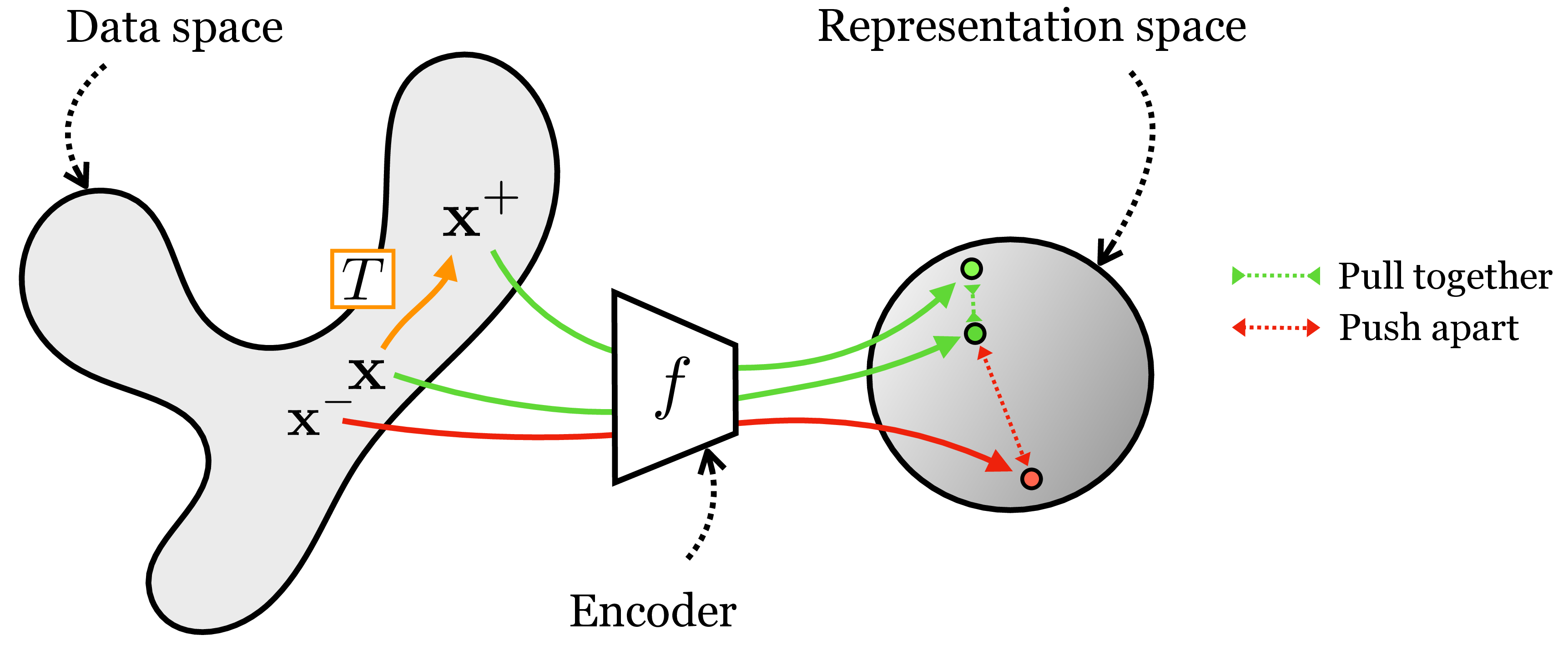
The idea is to simply penalize deviations from the invariance we want. Suppose \(T\) is a transformation we wish our representation to be invariant to. Then we may use a loss of the form \(\left\lVert f(T(\mathbf{x}))-f(\mathbf{x})\right\rVert_2^2\) to learn an encoder \(f\) that is invariant to \(T\). We call such a loss an alignment loss (wang2020hypersphere?).
That seems easy enough, but you may have noticed a flaw: What if \(f\) just learns to output the zero vector all the time? Trivial alignment can be achieved when there is representational collapse, and all datapoints get mapped to the same arbitrary vector.
Contrastive learning fixes this issue by coupling an alignment loss with a second loss that pushes apart embeddings of datapoints for which we do not want an invariant representation. The supervision for contrastive learning comes in the form of positive pairs and negative pairs. Positive pairs are two datapoints we wish to align in \(z\)-space; if we wish for invariance to \(T\) then a positive pair should be constructed as \(\{\mathbf{x}, \mathbf{x}^{+}\}\) with \(\mathbf{x}^{+} = T(\mathbf{x})\). Negative pairs, \(\{\mathbf{x},\mathbf{x}^-\}\), are two datapoints that should be represented differently in \(z\)-space. Commonly, negative pairs are randomly constructed by sampling two datapoints independently and identically from the same data distribution, that is, \(\mathbf{x} \sim p_{\texttt{data}}(\mathbf{x})\) and \(\mathbf{x}^{-} \sim p_{\texttt{data}}(\mathbf{x})\). Given such data pairings, the objective is to pull together the positive pairs and push apart the negative pairs, as illustrated in Figure 1.
This kind of contrastive learning results in an embedding that is invariant to a transformation \(T\). Extending this to achieve invariance to a set of transformations \(\{T_1, \ldots, T_n\}\) is straightforward: just apply the same loss for each of \(T_1, \ldots, T_n\).
A second kind of contrastive learning is based on co-occurrence, where the goal is to learn a common representation of all co-occurring signals. This form of contrastive learning is useful for learning, for example, an audiovisual representation where the embedding of an image matches the embedding of the sound for that same scene. Or, returning to our colorization example, we can learn an image representation where the embedding of the grayscale channels matches the embedding of the color channels. In both these cases we are learning to align co-occurring sensory signals. This kind of contrastive learning is schematized in Figure 2.
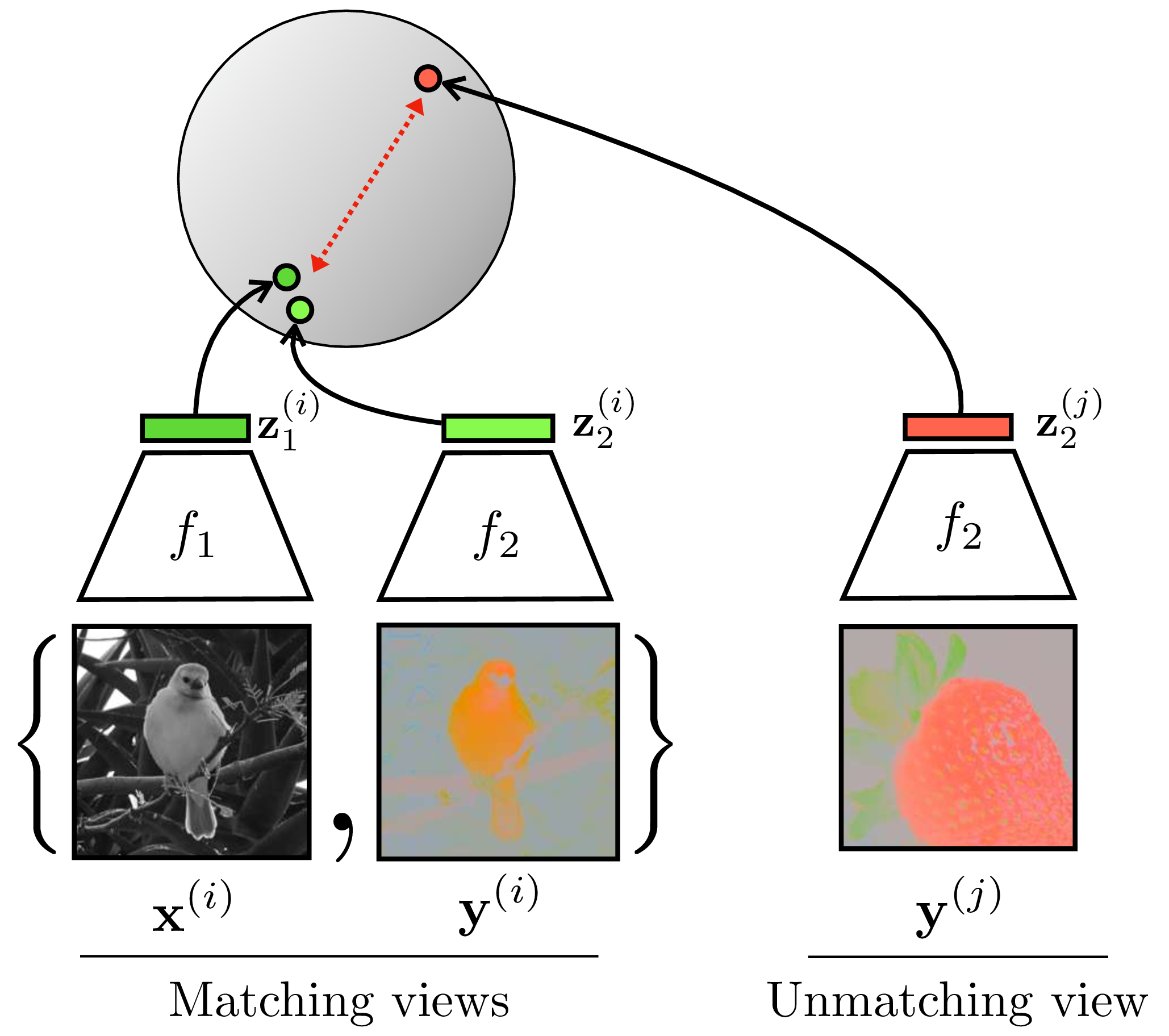
In Figure 2, we refer to the two co-occurring signals—color and grayscale—as two different views of the total data tensor \(\mathbf{X}\), just like we did in the previous sections: \(\mathbf{x} = V_1(\mathbf{X})\), \(\mathbf{y} = V_1(\mathbf{X})\). You can think of these views either as resulting from sensory co-occurrences or as two transformations of \(\mathbf{X}\), where the transformation in the color example is channel dropping. Thus, the two kinds of contrastive learning we have presented are really one and the same: any two signals can be considered transformations of a combined total signal, and any signal and its transformation can be considered two co-occurring ways of measuring the underlying world.
Nonetheless, it is often easiest to conceptualize these two approaches separately, and next we give learning diagrams for each:
![]()
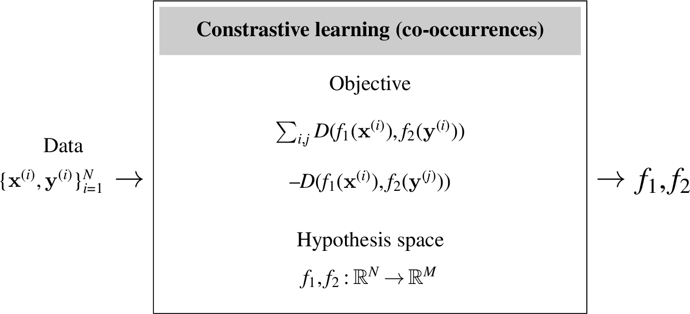
In these diagrams, \(D\) is a distance function. Above we give just one simple form for the contrastive objective; many variations have been proposed. Three of the most popular are (1) Hadsell et al.’s “constrastive loss” (hadsell2006dimensionality?) (an older definition of the term, now overloaded with our more general notion of a contrastive loss being the broader family of any loss that pulls together positive samples and pushes apart negative samples), (2) the triplet loss (chechik2010large?), and (3) the InfoNCE loss (oord2018representation?). Hadsell et al.’s contrastive loss and the triplet loss add the concept of a margin to the vanilla formulation: they only push/pull when the distance is less than a specified amount \(m\) (called the margin), otherwise points are considered far enough apart (or close enough together). The InfoNCE loss is a variation that treats establishing a contrast as a classification problem: it tries to move points apart until you can classify the positive sample, for a given anchor, separately from all the negatives. The general formulation of these losses takes as input an anchor \(\mathbf{x}\), a positive example \(\mathbf{x}^+\), and one or more negative examples \(\mathbf{x}^-\). The positive and negative may be defined based on transformations, coocurrences, or something else. The full learning objective is to sum over many samples of anchors, positives, and negatives, producing a sampled set evaluated according to the losses as follows: \[\begin{aligned} \mathcal{L}(\mathbf{x}, \mathbf{x}^+, \mathbf{x}^-) &= \max(D(f(\mathbf{x}), f(\mathbf{x}^+)-m_{\texttt{pos}},0) - \nonumber \\ &\quad \max(m_{\texttt{neg}} - D(f(\mathbf{x}), f(\mathbf{x}^-),0) \quad \triangleleft \quad \text{Hadsell et al. ``contrastive''}\\ \mathcal{L}(\mathbf{x}, \mathbf{x}^+, \mathbf{x}^-) &= \max(D(f(\mathbf{x}), f(\mathbf{x}^+)) - D(f(\mathbf{x}), f(\mathbf{x}^-)) + m, 0) \quad\quad \triangleleft \quad \text{triplet}\\ \mathcal{L}(\mathbf{x}, \mathbf{x}^+, \{\mathbf{x}_i^-\}_{i=1}^N) &= -\log \frac{e^{f(\mathbf{x})^\mathsf{T}f(\mathbf{x}^+)/\tau}}{e^{f(\mathbf{x})^\mathsf{T}f(\mathbf{x}^+)/\tau} + \sum_i e^{f(\mathbf{x})^\mathsf{T}f(\mathbf{x}_i^-)/\tau}} \quad\quad\quad\quad\quad\quad\triangleleft \quad \text{InfoNCE} \end{aligned} \tag{1}\] Notice that the InfoNCE loss is a log softmax over a vector of scores \(f_1(\mathbf{x})^\mathsf{T}f_2(c)/\tau\) with \(c \in \{\mathbf{x}^+, \mathbf{x}_1^-, \ldots, \mathbf{x}_N^-\}\); you can therefore think of this loss as corresponding to a classification problem where the ground truth class is \(\mathbf{x}^+\) and the other possible classes are \(\{\mathbf{x}_1^-, \ldots, \mathbf{x}_N^-\}\) (refer to ?@sec-intro_to_learning to revisit softmax classification).
Alignment and Uniformity
Wang and Isola (wang2020hypersphere?) showed that the contrastive loss (specifically the InfoNCE form) encourages two simple properties of the embeddings: alignment and uniformity. We have already seen that alignment is the property that two views in a positive pair will map to the same point in embedding point, that is, the mapping is invariant to the difference between the views. Uniformity comes from the negative term, which encourages embeddings to spread out and tend toward an evenly spread, uniform distribution. Importantly, for this to work out mathematically, the embeddings must be normalized, that is, each embedding vector must be a unit vector. Otherwise, the negative term can push embeddings toward being infinitely far apart from each other. Fortunately, it is standard practice in contrastive learning (and many other forms of representation learning) to apply \(L_2\) normalization to the embeddings. The result is that the embeddings will tend toward a uniform distribution over the surface of the \(M\)-dimensional hypersphere, where \(M\) is the dimensionality of the embeddings. See theorem 1 in (wang2020hypersphere?) for a formal statement of this fact.
A result of this analysis is we may explicit decompose contrastive learning into one loss for alignment and another for uniformity, with the following forms: \[\begin{aligned} \mathcal{L}_{\texttt{align}}(f;\alpha) &= \mathbb{E}_{(\mathbf{x},\mathbf{x}^+) \sim p_{\texttt{pos}}} [\left\lVert f(\mathbf{x}) - f(\mathbf{x}^+)\right\rVert_2^{\alpha}]\\ \mathcal{L}_{\texttt{unif}}(f;t) &= \log \mathbb{E}_{\mathbf{x} \sim p_{\texttt{data}}, \, \mathbf{x}^- \sim p_{\texttt{data}}} [e^{-t\left\lVert f(\mathbf{x}) - f(\mathbf{x}^-)\right\rVert_2^2}]\\ \mathcal{L}(f;\alpha,t,\lambda) &= \mathcal{L}_{\texttt{align}}(f;\alpha) + \lambda \mathcal{L}_{\texttt{unif}} \end{aligned}\] where \(p_{\texttt{pos}}\) is the distribution of positive pairs and \(\alpha\), \(t\), and \(\lambda\) are hyperparameters of the losses.
CLIP Architecture
Here, we use the pretext task idea on a supervisory signal of the natural language to create a representation of the scene it describes.
CLIP is a contrastive method (see ?@sec-representation_learning-contrastive_learning) in which one data view is the image and the other is a caption describing the image. Specifically, CLIP is a form of contrastive learning from co-occurring visual and linguistic views that is formulated as follows:
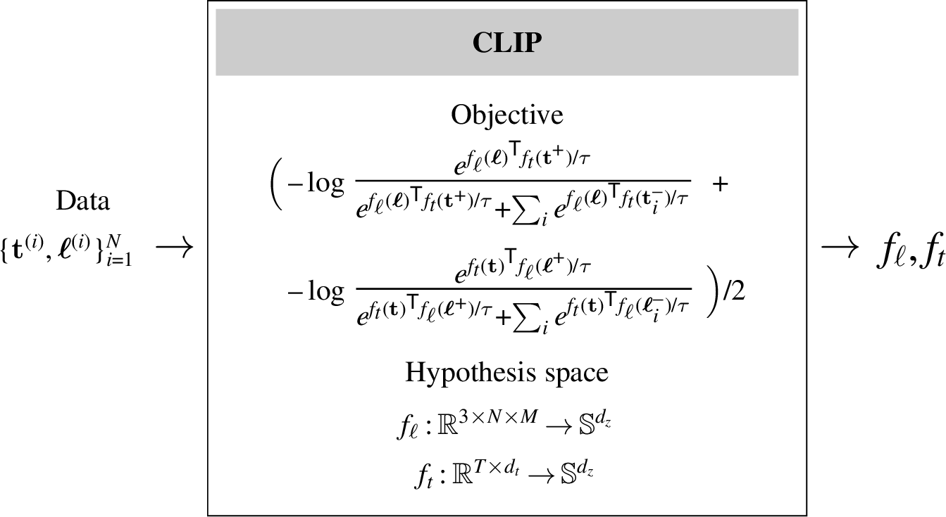
where \(\boldsymbol\ell\) represents an image, \(\mathbf{t}\) represents text, \(\mathbb{S}^{d_z}\) represents the space of unit vectors of dimensionality \(d_z\) (i.e., the surface of the \([d_z-1]\)-dimensional hypersphere), \(f_{\ell}\) is the image encoder, \(f_t\) is the text encoder, image inputs are represented as \([3 \times N \times M]\) pixel arrays, text inputs are represented as \(d_t\) dimensional tokens, and \(d_z\) is the embedding dimensionality. Notice that the objective is a symmetric version of the InfoNCE loss defined in Equation 1. Also notice that \(f_\ell\) and \(f_t\) both output unit vectors (which is achieved using \(L_2\)-normalization before computing the objective); this ensures that the denominator cannot dominate by pushing negative pairs infinitely far apart.
The idea of visual learning by image captioning actually has a long history before CLIP. One important early paper on this topic is (ordonez2011im2text?).
Figure 3 visually depicts how CLIP is trained. First we sample a batch of \(N\) language-image pairs, \(\{\mathbf{t}^{(i)}, \boldsymbol\ell^{(i)}\}_{i=1}^N\) (\(N=6\) in the figure). Next we embed measure the dot product between all these text strings and images using a language encoder \(f_t\) and an image encoder \(f_\ell\), respectively. This produces a set of text embeddings \(\{\mathbf{z}^{(i)}_t\}_{i=1}^N\) and a set of image embeddings \(\{\mathbf{z}^{(i)}_\ell\}_{i=1}^N\). To compute the loss, we take the dot product \(\mathbf{z}^{(i)}_\ell\cdot \mathbf{z}^{(j)}_t\) for all \(i, j \in \{1,\ldots,6\}\). Terms for which \(i \neq j\) are the negative pairs and we seek to minimize these dot products (denominator of the loss); terms for which \(i == j\) are the positive pairs and we seek to maximize these dot product (they appear in both the numerator and denominator of the loss).
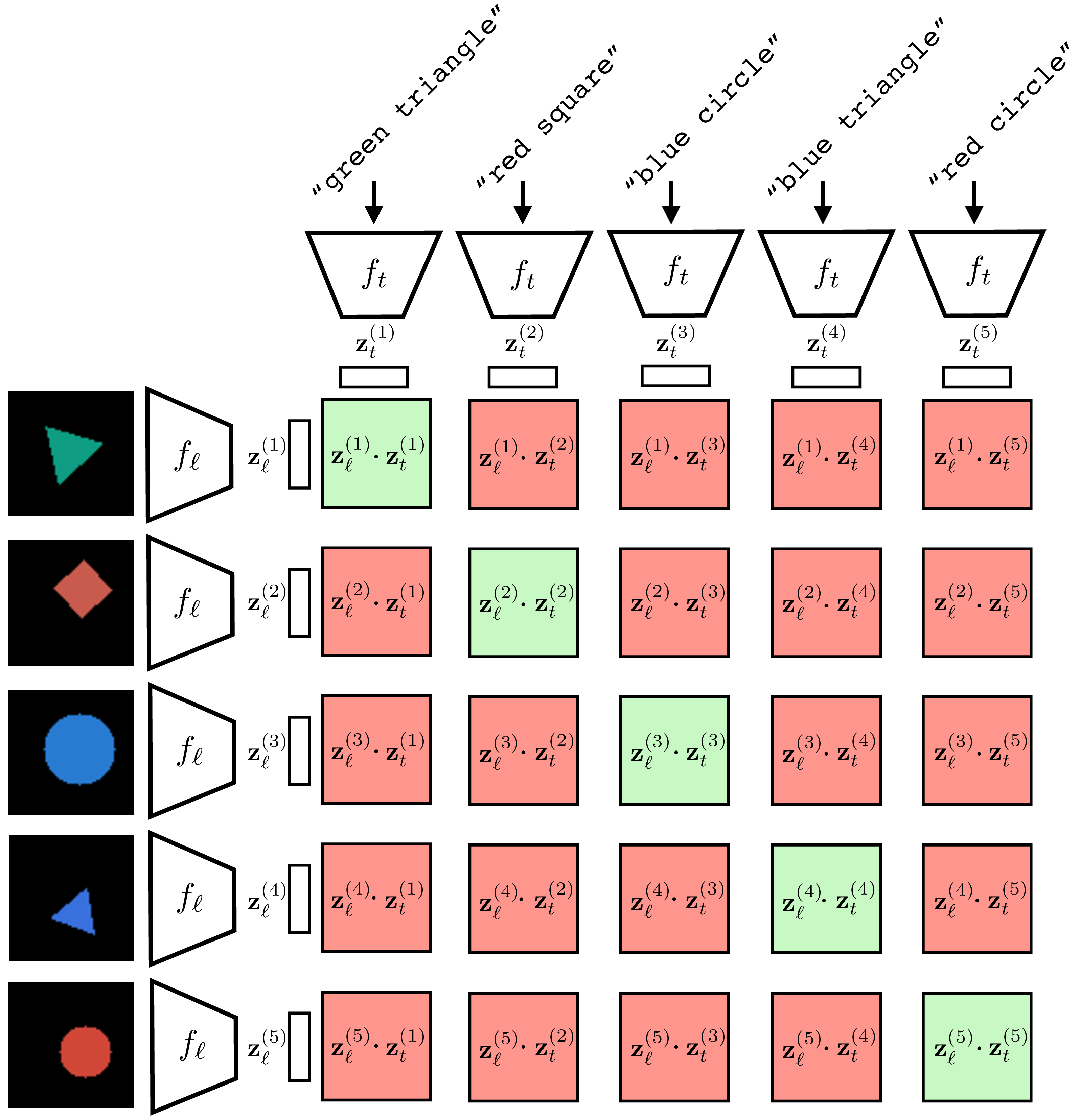
After training, we have a text encoder \(f_t\) and an image encoder \(f_\ell\) that map to the same embedding space. In this space, the angle between a text embedding and an image embedding will be small if the text matches the matches.
The dot product between unit vectors is proportional to the angle between the vectors.
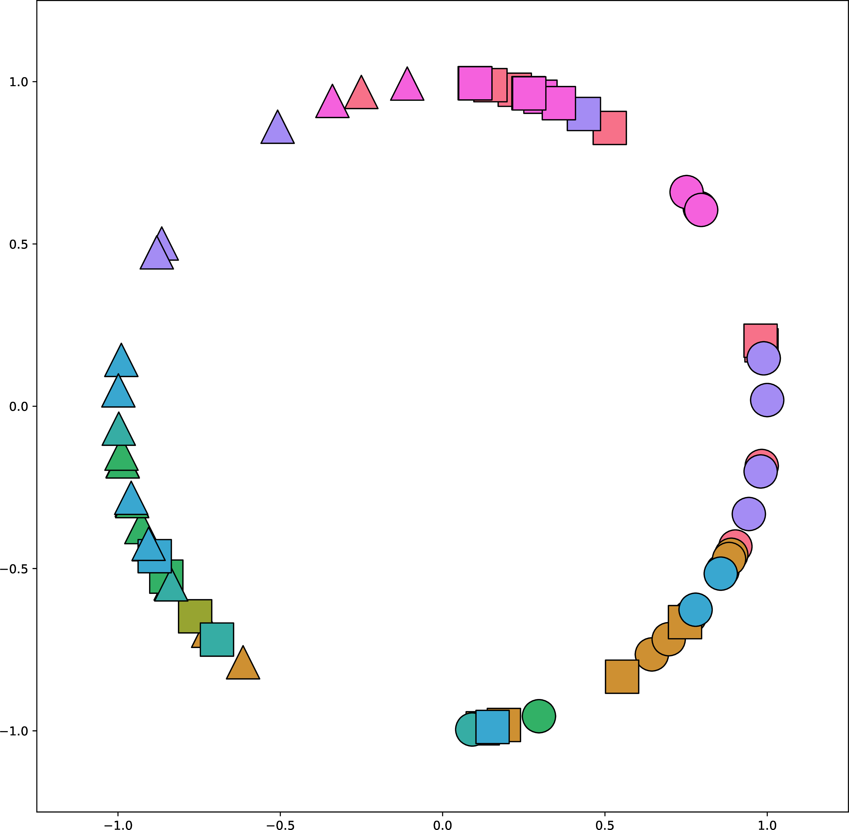
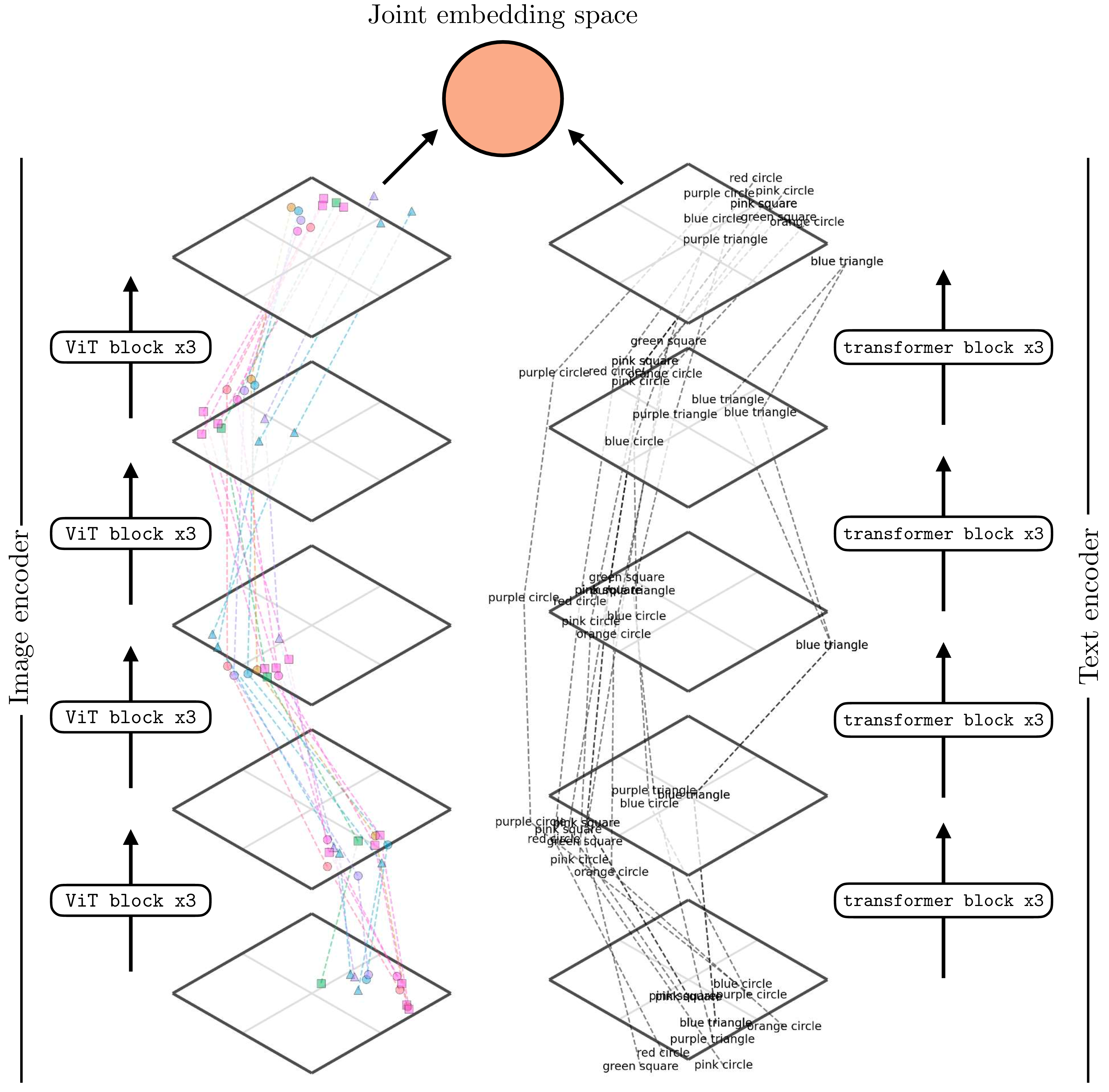
Figure 4 shows how a trained CLIP model maps data to embeddings. This figure is generated in the same way as ?@fig-neural_nets-vit_mapping_plot: for each encoder we reduce dimensionality for visualization using t-distributed Stochastic Neighbor Embedding (t-SNE) (tsne?). For the image encoder, we show the visual content using icons to reflect the color and shape depicted in the image (we previously used the same visualization in ?@sec-representation_learning-expt_designing_embeddings_with_contrastive_learning).
It’s a bit hard to see, but one thing you can notice here is that for the image encoder, the early layers group images by color and the later layers group more by shape. The opposite is true for the text encoder. Why do you think this is? One reason may be that color is a superficial feature in pixel-space while shape requires processing to extract, but in text-space, color words and shape words are equally superficial and easy to group sentences by.
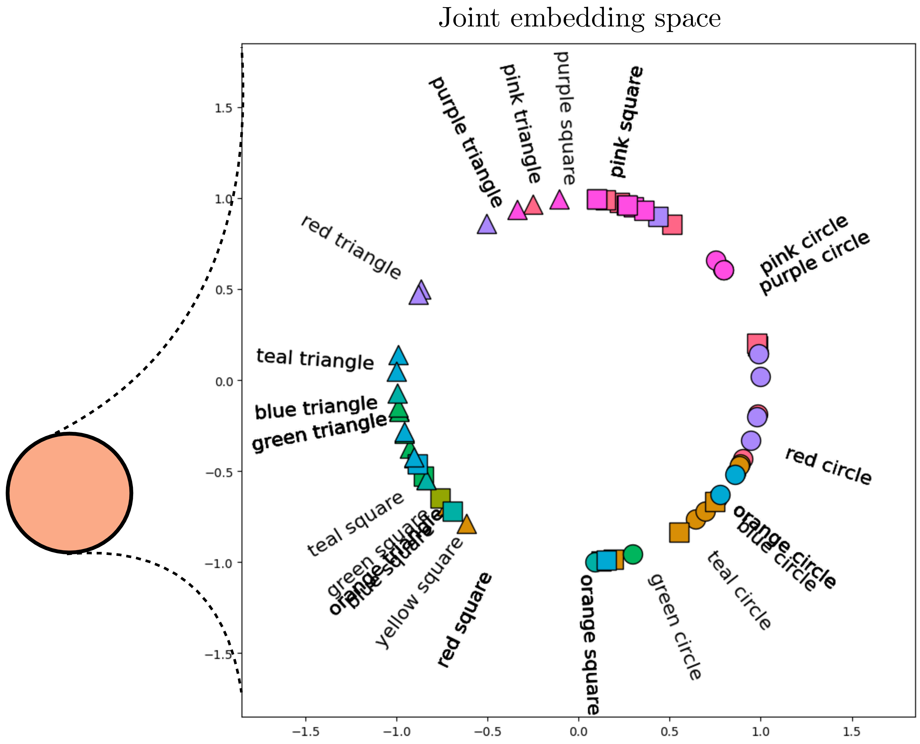
After passing the data through these two encoders, the final stage is to normalize the outputs and compute the alignment between the image and text embeddings. Figure 5 shows this last step. After normalization, all the embeddings line on the surface of a hypersphere (the circle in the figure). Notice that the text descriptions are embedded near the image embeddings (icons) that match that description. It’s not perfect but note that this is partially due to limitations in the visualization, which projects the \(768\)-dimensional CLIP embeddings into a 2D visualization. Here we use kernel principle component analysis (scholkopf1998nonlinear?) on the embeddings, with a cosine kernel, and remove the first principle component as that component codes for a global offset between the image embeddings and text embeddings.
Using language as one of the views may seem like a minor variation on the contrastive methods we saw previously, but it’s a change that opens up a lot of new possibilities. CLIP connects the domain of images to the domain of language. This means that many of the powerful abilities of language become applicable to imagery as well. One ability that the CLIP paper showcased is making a novel image classifier on the fly. With language, you can describe a new conceptual category with ease. Suppose I want a classifier to distinguish striped red circles from polka dotted green squares. These classes can be described in English just like that: “striped red circles” versus “polka dotted green square.” CLIP can then leverage this amazing ability of English to compose concepts and construct an image classifier for these two concepts.
Here’s how it works. Given a set of sentences \(\{\mathbf{t}^{a}, \mathbf{t}^{b}, \ldots\}\) that describe images of classes \(a\), \(b\), and so on,
Embed each sentence into a \(\mathbf{z}\)-vector, \(\mathbf{z}_t^{a} = f_t(\mathbf{t}^{a}), \mathbf{z}_t^{b} = f_t(\mathbf{t}^{a}),\) and so on.
Embed your query image into a \(\mathbf{z}\)-vector, \(\mathbf{z}_{\ell}^{q} = f_{\ell}(\boldsymbol\ell^{q})\).
See which sentence embedding is closest to your image embedding; that’s the predicted class.
These steps are visualized in Figure 6. The green outlined dot product is the highest, indicating that the query image will be classified as class \(a\), which is defined as “striped red circles.”
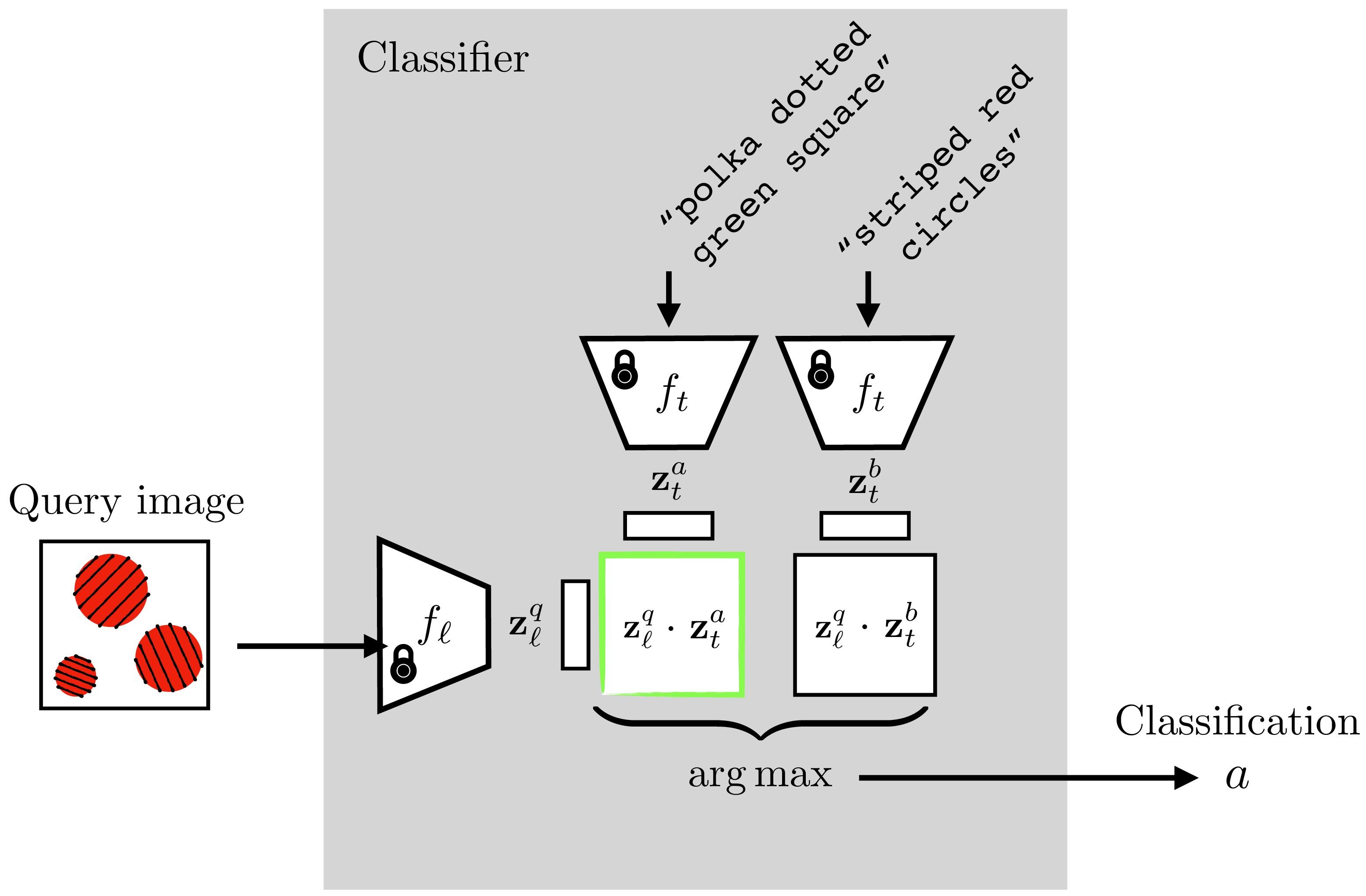
striped red circles'' (class $a$) versuspolka dotted green square’’ (class \(b\)) classifier using a trained CLIP. The CLIP model parameters are frozen and not updated. Instead the classifier is constructed by embedding the text describing to the two classes and seeing which is closer to the embedding of the query image. Inspired by figure 1 of (radford2021learning?)
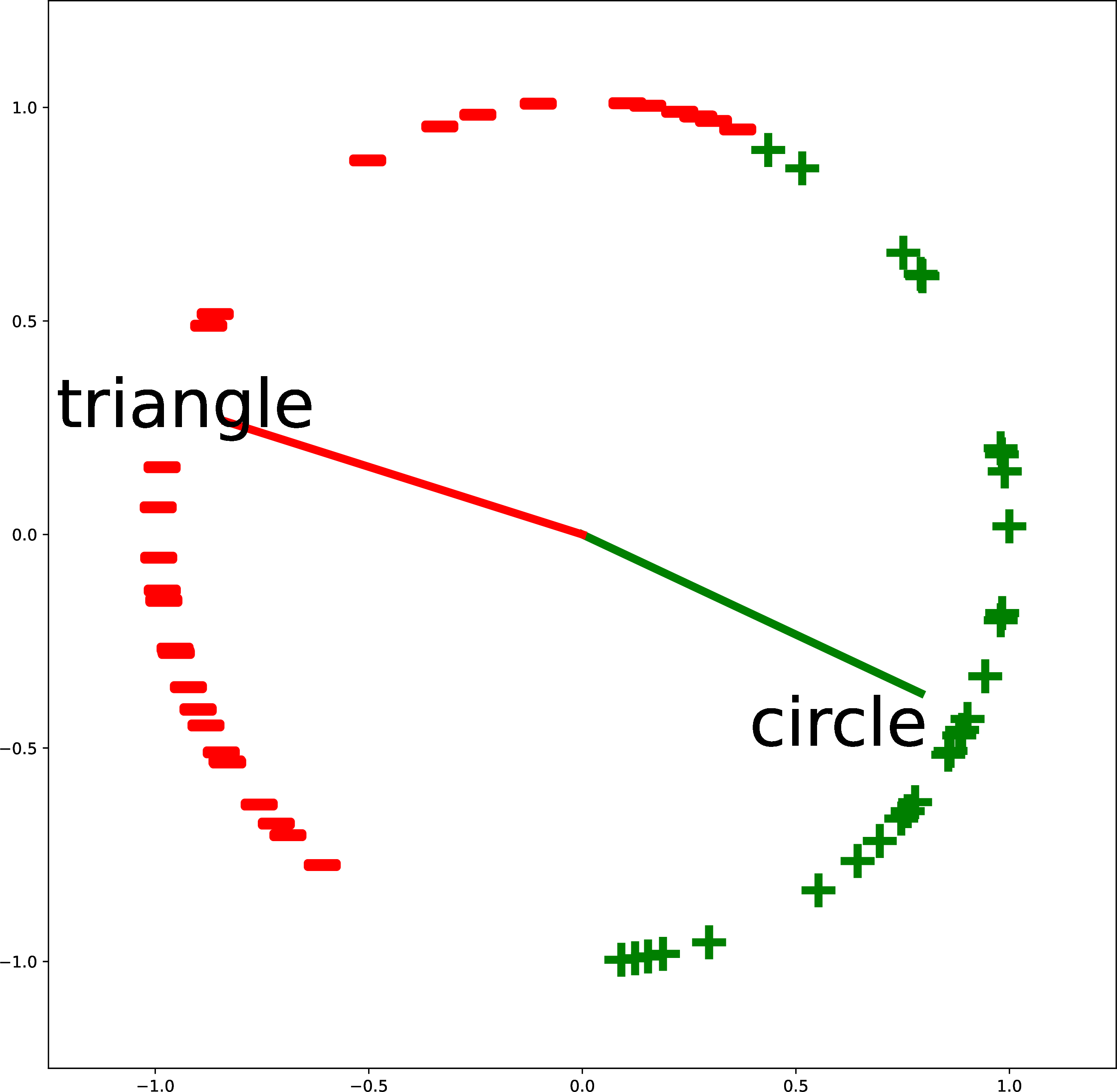
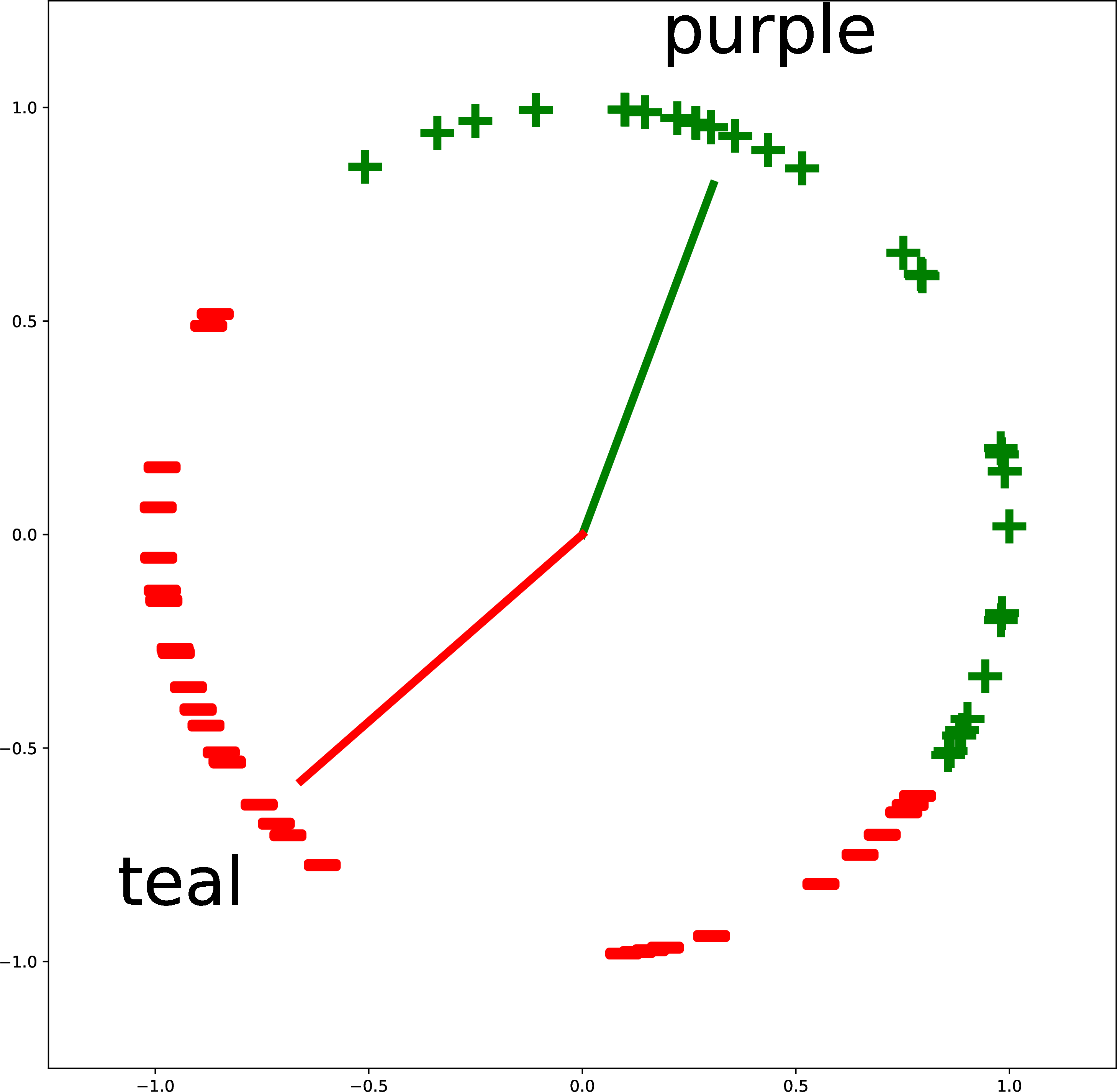
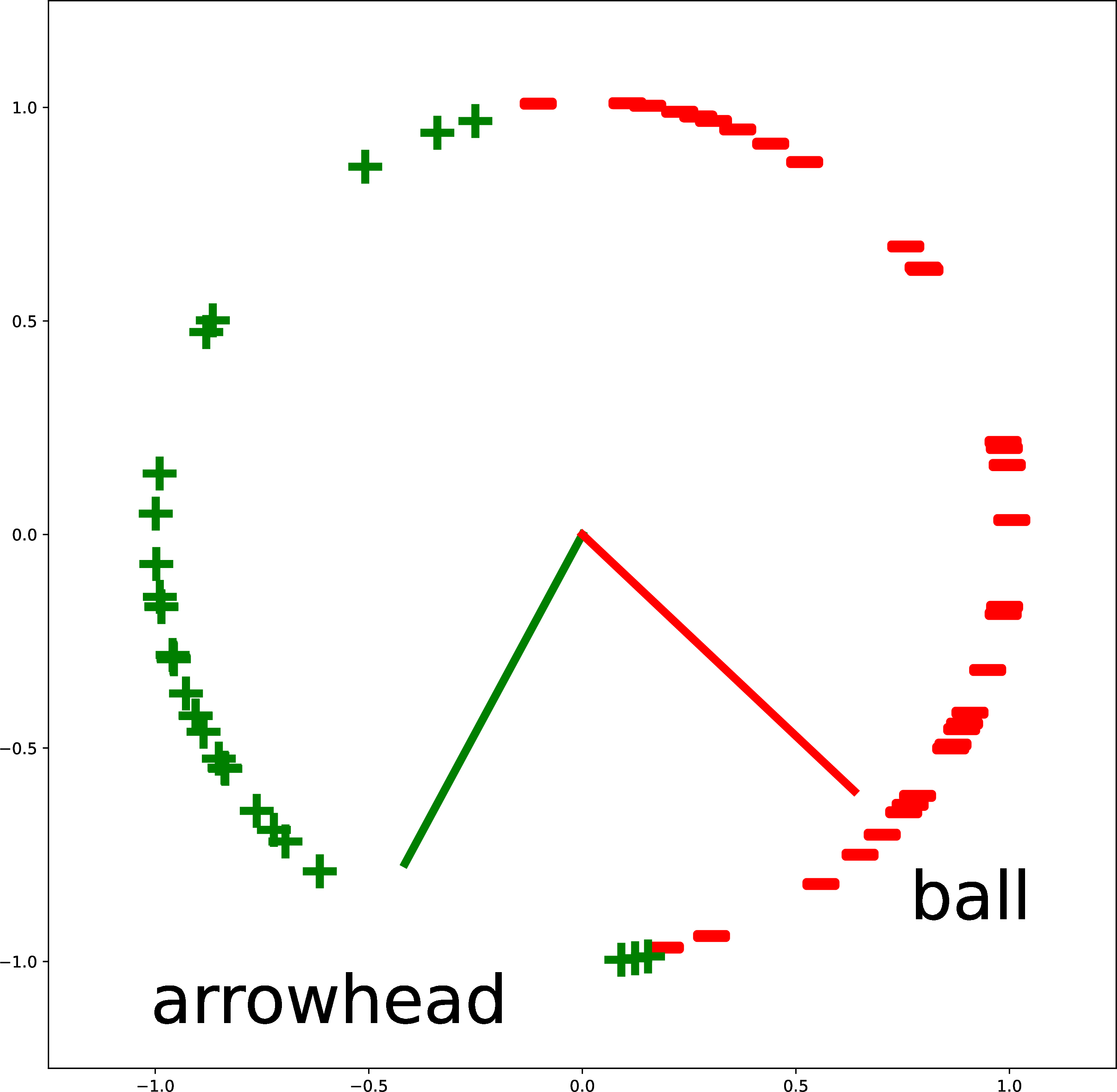
Figure 7 gives more examples of creating custom binary classifiers in this way. The two classes are described by two text strings (“triangle” versus “cricle”; “purple” versus “teal”; and “arrowhead” versus “ball”). The embeddings of the text descriptions are the red and green vectors. The classifier simply checks where an image embedding is closer, in angular distance, to the red vector or the green vector. This approach isn’t limited to binary classification: you can add more text vectors to partition the space in more ways.