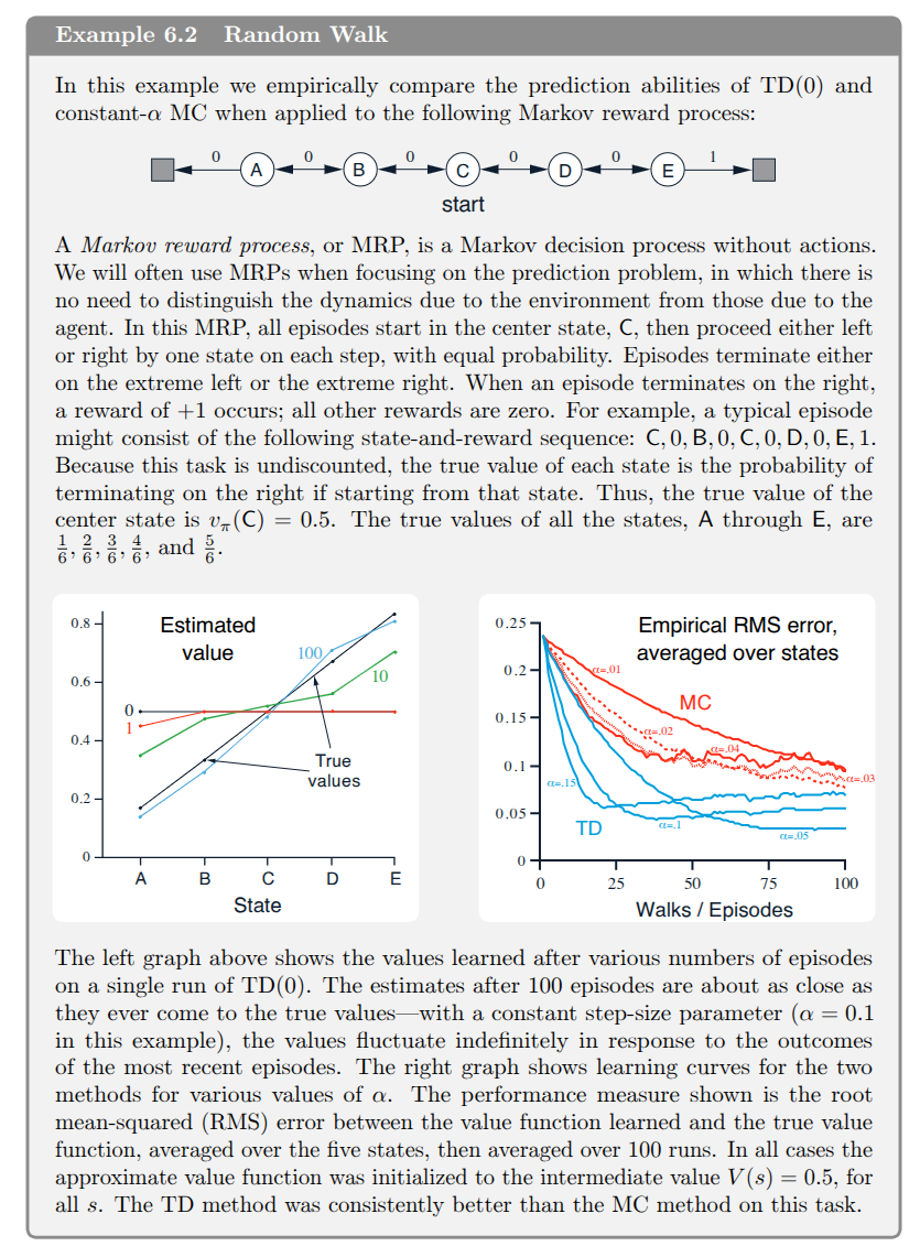
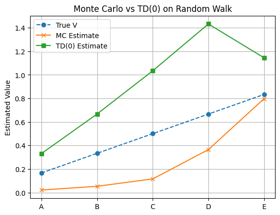
It is instructive to see the difference between MC and TD approaches in the following example.
import numpy as np
import matplotlib.pyplot as plt

states = ['A', 'B', 'C', 'D', 'E']
state_to_index = {s: i for i, s in enumerate(states)}
n_states = len(states)

def generate_episode(start='C'):
    state = state_to_index[start]
    episode = []
    while True:
        action = np.random.choice([-1, 1])  # left or right
        next_state = state + action
        if next_state < 0:
            return episode + [(state, 0)]  # Left terminal, reward 0
        elif next_state >= n_states:
            return episode + [(state, 1)]  # Right terminal, reward 1
        else:
            episode.append((state, 0))
            state = next_state

def mc_prediction(episodes=1000, alpha=0.1):
    V = np.full(n_states, 0.5)
    #V = np.zeros(n_states)
    for _ in range(episodes):
        episode = generate_episode()
        G = episode[-1][1]  # Only final reward matters
        for (s, _) in episode:
            V[s] += alpha * (G - V[s])
    return V

def td0_prediction(episodes=10000, alpha=0.01):
    #V = np.zeros(n_states)
    V = np.full(n_states, 0.5)

    for _ in range(episodes):
        episode = generate_episode()
        for i in range(len(episode) - 1):
            s, _ = episode[i]
            s_next, r = episode[i + 1]
            V[s] += alpha * (r + V[s_next] - V[s])
        # final transition
        s, r = episode[-1]
        V[s] += alpha * (r - V[s])
    return V

# Run both methods
V_mc = mc_prediction()
V_td = td0_prediction()

# Ground truth (analytical solution): [1/6, 2/6, 3/6, 4/6, 5/6]
true_V = np.array([1, 2, 3, 4, 5]) / 6

# Plot results
plt.plot(true_V, label='True V', linestyle='--', marker='o')
plt.plot(V_mc, label='MC Estimate', marker='x')
plt.plot(V_td, label='TD(0) Estimate', marker='s')
plt.xticks(ticks=range(n_states), labels=states)
plt.ylabel("Estimated Value")
plt.title("Monte Carlo vs TD(0) on Random Walk")
plt.legend()
plt.grid(True)
plt.show()