Variational Inference

Introduction

In probabilistic graphical modeling we saw the necessity of latent representations. In this section we advance the topic to the case where we need to learn features that are suitable for generating data from a complex data distribution.

After reviewing the premise of generative modeling via what we will call deep latent variable models, we will look at the problem of inference of the latent space that is suitable for generating such data. We will see that this problem is intractable and we will introduce the variational inference method that will allow us to approximate the posterior distribution of the latent space.

The method that we will dive into is called Variational Autoencoder (VAE) that is used across various domains, including collaborative filtering, image compression, reinforcement learning, and generation of content such as music and images. VAEs can also serve as the base to understand advanced topics such as Stable Diffusion Models (SDMs) that are used in the generation of images and videos.

We will focus on continuous VAEs in this edition of the course.

Calculus of Variations

One of the main methods of generative approximate inference is variational inference that originates from calculus of variations. To understand how this calculus differs from the one we are used to, consider how the standard calculus using the derivative of a function is able to optimize it and calculate its minimum. In a similar way, in calculus of variations we are able to optimize a functional. A functional in mathematics is a mapping from a function space to the real numbers - just like the function is a mapping from a real number (the argument) to a real value (the result of the function evaluation).

The concept of a functional can be illustrated with the definition of entropy, in the context of information theory.

Shannon entropy, denoted as \(H\), is a measure of the uncertainty or randomness in a probability distribution. It’s defined for a discrete probability distribution \(P = (p_1, p_2, \ldots, p_n)\), where \(p_i\) is the probability of the \(i\)-th outcome. The entropy is defined as:

\[ H(P) = -\sum_{i=1}^{n} p_i \log p_i \]

Here, \( H \) is a functional because it maps the function (in this case, the probability distribution function \(P\) to a real number, which represents the entropy of \(P\).

The calculus of variations is concerned with finding the function that maximizes a functional. In the case of entropy, the function that maximizes the entropy is the uniform distribution, where all the outcomes have the same probability. This is intuitive, because if all the outcomes have the same probability, then we have the most uncertainty about the outcome.

The Variational Generative Modeling Problem

VAE is one of the answers to the aforementioned variational optimization problem. In this approach, we use a neural network to create the right structure instead of explicitly encoding it in the prior.

This is not a new idea - sampling from a complex probability distribution can be achieved by feeding samples from a simple distribution to a suitably chosen function. In the example below, the a function is used to change the mean of the standard normal distribution to generate a half-moon shape.

import numpy as np
import matplotlib.pyplot as plt

def generate_half_moon(num_points, radius, width):
    
    # Generate points on a circle
    theta = np.linspace(0, np.pi, num_points)
    x_circle = radius * np.cos(theta)
    y_circle = radius * np.sin(theta)

    # The function changes the mean of the standard normal distribution
    x_noisy = x_circle + np.random.normal(0, width, num_points)
    y_noisy = y_circle + np.random.normal(0, width, num_points)

    # Combine x and y coordinates
    half_moon_points = np.column_stack((x_noisy, y_noisy))

    return half_moon_points

# Example usage:
half_moon_data = generate_half_moon(num_points=1000, radius=1.0, width=0.1)

plt.scatter(half_moon_data[:, 0], half_moon_data[:, 1])
plt.xlabel("X-axis")
plt.ylabel("Y-axis")
plt.title("Generated Half-Moon")
plt.show()

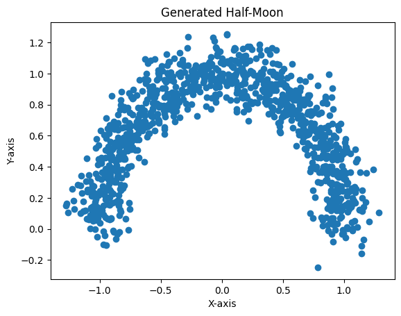
The neural network is abstracting such function and we can now see a path to implemeting the aforementioned generator,

\[ p(\mathbf x | \mathbf \theta) = \sum_{\mathbf z} p(\mathbf x| \mathbf z ; \mathbf \theta) p(\mathbf z | \theta)\]

by assuming that the conditional distribution \(p(\mathbf x| \mathbf z ; \mathbf \theta)\) is parameterized by a neural network that takes as input the latent vector \(\mathbf z\) generated itself by the prior distribution and outputs the image \(\mathbf x\).

In the case that the \(p(\mathbf x| \mathbf z ; \mathbf \theta)\) is Gaussian, this will mean:

\[ p(\mathbf x| \mathbf z ; \mathbf \theta) = N(\mathbf x; \mu(\mathbf z; \mathbf \theta), \sigma^2 \mathbf I)\]

where \(\mu(\mathbf z; \mathbf \theta)\) is the output of the neural network that is parameterized by \(\mathbf \theta\). Note that the variance of the Gaussian is fixed, is a hyperparameter and is not a function of \(\mathbf z\).

Note that the \(p(\mathbf x| \mathbf z ; \mathbf \theta)\) can be any distribution and obviosuly this distribution need to match the nature of what we try to generate. If \(\mathbf x\) is binary then this can be a Bernouli distribution with the parameter(s) of the distribution given at the output of the neural network.

The Optimization Problem and Objective

However there is a problem with this generator. Even with neural networks “designing” the right features in the latent space [2], we are still facing a very heavy computationally problem in trying to estimate the marginal distribution \(p(\mathbf x | \mathbf \theta)\).

To understand why, consider the MNIST dataset and the problem of generating handwritten digits that look like that. We can sample from \(p(\mathbf z | \theta)\) generating a large number of samples \(\{z_1, \dots , z_m\}\), and with the help of the neural network sample and compute \(p(\mathbf x) = \frac{1}{m} \sum_i p(\mathbf x|z_i)\).

The problem is that we need a very large number of such samples in high dimensional spaces such as images (for MNIST is 28x28 dimensions) . Most of the samples \(\mathbf z_i\) will result into negligible \(p(\mathbf x|z_i)\) and therefore won’t contribute to the estimate of the \(p(\mathbf x)\).

This is the problem that VAE addresses. The key idea behind its design is that of inference of the right latent space such that when \(\mathbf z\) is sampled, it results into a \(\mathbf x\) that is very similar to that of our training data. VAE in other works buys us sample efficiency allowing computation and optimization of the objective function with far less effort than before.

References

[1]: Diederik Kingma and Max Welling. Auto-Encoding Variational Bayes. In International Conference on Learning Representations, 2014, https://arxiv.org/abs/1312.6114

[2]: Yuri Burda, Roger Grosse, Ruslan Salakhutdinov. Importance Weighted Autoencoders. In International Conference on Learning Representations, 2015, https://arxiv.org/abs/1509.00519

---

[2]

Note that the features that the neural network captures are not interpretable as the intuitively understood features that humans consider. For the MNIST dataset for example, humans will consider the slant of each digit, thinner strokes etc.