Generative Modeling and Probabilistic Graphical Modeling#
Generative models#
In generative modeling we want to model the generative distribution of the observed variables \(\mathbf x\), \(p(\mathbf x)\) [1].
Take for example a set of images that depict a pendulum excited by a force. We would like to generate the successive frames of the pendulum swinging behavior and we do so we are assisted by a set of latent variables \(\mathbf z\) that represent the underlying laws of physics. Generative modeling is especially well suited for:
Testing out hypotheses about the underlying rules that generated the observed data. Such rules can also offer interpretable models.
Ability to capture causal relationships, since the ability of a factor to generate data very close to the ones observed, offers a strong indication of such relationship.
Semi-supervised learning where the generated data are very close to already labeled data and therefore can improve classification model accuracy.
The use of latent variables \(\mathbf z\), that are not observed but can be used to build suitable representational constraints in our models, and a set of parameters \(\theta\) that parametrize the latent variable model \(p(\mathbf x, \mathbf z | \mathbf \theta)\) is more formally presented using an example of generating realistic images of people’s faces. We can think of the problem as a two step process:
Think of what factor make a person a real one. For example, can we have a person without a head (assume we are interested in living humans) ? Lets call the headedness factor a latent variable and similarly specify the other factors grouping them together into a set of rendom variables that we will call \(\mathbf z\), captured via their distribution \(p(\mathbf z | \theta)\).
Generate an image from the latent representation. This is a process that takes the latent representation and generates an image of the person (hopefully realistic).
Since,
to generate new data whose marginal is ideally, identical to the true but unknown target distribution we need to be able to sample from \(p(\mathbf x, \mathbf z | \mathbf \theta)\). Equivalently, after applying the prodcut rule we have:
The elements of this model are \(p(\mathbf x| \mathbf z ; \mathbf \theta)\) and the \(p(\mathbf z | \theta)\) that is often called the prior distribution over \(\mathbf z\).
Note that for continuous variables, the sum is replaced by an integral.
Probabilistic Graphical Models#
A graph representation, the Probabilistic Graphical Model (PGM) (also called Bayesian network) can be used to capture dependencies between the random variables involved in the modeling of a problem. We can use such representations to efficiently compute conditional probabilities using the graph to identify the conditionally independent random variables that are present in our problem.
By convention, we represent PGMs as directed graphs, with nodes being the random variables involved in the model and directed edges indicating a parent child relationship, with the arrow pointing to a child, representing that the child nodes are probabilistically conditioned on the parent(s). We have assumed that our model does not have variables involved in directed cycles and therefore we call such graphs Directed Acyclic Graphs (DAGs).
In a hypothetical example of a joint distribution with \(K=7\) random variables,
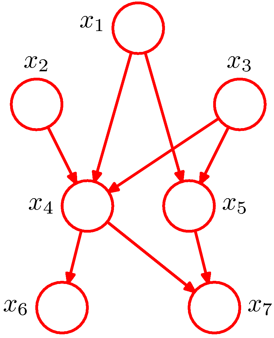
The PGM above represents the joint distribution \(p(x_1, x_2, ..., x_7)=p(x_1)p(x_2)p(x_3)p(x_4|x_1, x_2, x_3)p(x_5|x_1, x_3) p(x_6|x_4)p(x_7|x_4, x_5)\). In general,
where \(\mathtt{pa}_k\) is the set of parents of node \(x_k\).
An example is now in order for us to be able to ground the discussion up to now. In our attempt to generate realistic images of people’s faces we may consider a number of latent factors that can affect the image.
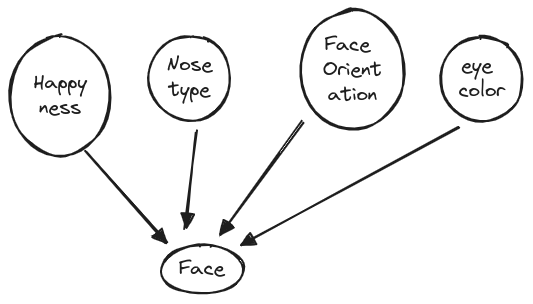
The shown latent factors are grouped together into a latent vector \(\mathbf z\), without an explicit semantic (or interpretable) mapping of each factor to the corresponding dimension of the \(\mathbf z\) vector. Further, we will assume that although there is an underlying structure, for example the happyness and face orientation are correlated since people when they laugh they tend to lift their chin up, such structure will not be explicitly captured a priori. To map this application to what were presenting as the generative PGM, the happiness and other latent factors are captured by a simple to generate Gaussian prior distribution:
Using a PGM we can represent the generative model we are concerned with, as shown below:
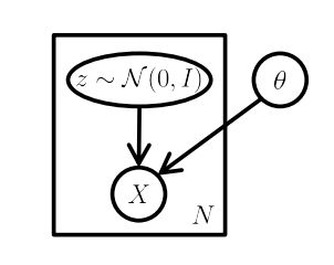
Probabilistic Graphical Model showing the model governing the generation of \(m\) samples from the probability distribution \(p(\mathbf x|\theta)\) - ref