Figure 1: Perspective projection and point at infinity where tracks intersect at the horizon.
As understood commonly by hundreds of pictures that each one of us have taken, projective geometry arises from a transformation - from the familiar 3D Euclidean space that we associated with the real world onto a 2D space, that of each picture. From our experience, circles in 3D Euclidean space are not preserved in the 2D space as they show up as ellipses and the same can be said about distances, angles, ratios of distances. We are also very familiar with straight lines are preserved and how parallel lines in Euclidean space are shown as intersecting as for example in this picture.
We can define a projective space as an extension of the Euclidean space where two lines always intersect at some point but some lines (parallel lines) intersect at infinity. We call a space homogenous when all its points are the same - this is true for both the classical Euclidean space as well as its extension the projective space. When coordinates are added in such spaces, seemingly we are picking out for the case of Euclidean spaces a “special” point and call it the origin but this does not change the homogenous nature of the space in that any point can be the origin.
Figure 2: In 2D, the coordinates of a point are defined by the relationship of the point to a particular 2D coordinate system. Here, two coordinate systems are shown; the point might have some coordinates with respect to the coordinate system with its coordinate axes drawn in solid lines but have different coordinates with respect to the coordinate system with dashed axes. In either case, the 2D point is at the same absolute position in space.
In the picture above we have seen two different frames each defined as a point of origin and two linearly independent basis vectors that define the axes of the 2-space. In general, the frame’s origin \(p_o\) and its \(n\) linearly indepedent basis define an n-dimensional affine frame. In this space for any vector \(\mathbf v\) there is a unique set of scalars \(s_i\) such as
where \(\mathbf s\) is a vector of coordinates. The vector \(\mathbf s\) is also called the representation of \(\mathbf v\) with respect to the frame aka with respect to the origin and the basis vectors. Similarly, for all points , there are unique scalars \(s_i\) such that the point can be expressed in terms of the origin \(p_o\) and the basis vectors,
An affine space of dimension \(n\) is a set of points, say \(\mathcal{A}\) together with an associated vector space \(V\) of dimension \(n\). It is equipped with two operations:
Point subtraction: \(p - q \in V\) (gives a vector)
Point translation: \(p + v \in \mathcal{A}\) (moves a point by a vector)
There is no fixed origin, no preferred coordinate system, and no basis until you choose one.
A coordinate frame on an affine space is a chosen origin point \(p_0 \in \mathcal{A}\) and a basis \(\{v_1, \dots, v_n\}\) for the associated vector space \(V\).
A vector space on the other hand has a built-in origin (defined by the zero vector) and supports linear combinations: \(a\mathbf{v}_1 + b\mathbf{v}_2\) being also closed under addition and scalar multiplication. This is the reason that it is also called a linear space. Notice that in an affine space you cannot add two points directly, like you do in vector spaces and there’s no zero point.
The Euclidean space adds inner product (so you can measure angles and lengths).
Thus, although points and vectors are both represented by x, y, and z coordinates in 3D, they are distinct mathematical entities and are not freely interchangeable. This is an important observation that lead us to act to resolve this ambiguity in their representation. Given a 3D frame for example, defined by \((p_o, \mathbf u_1, \mathbf u_2, \mathbf u_3)\), there is ambiguity between the representation of a point \((p_x, p_y, p_z)\) and a vector \((v_x, v_y, v_z)\) with the same coordinates. Using the representations of points and vectors introduced above, we can write the point as the inner product
The representation of points \([s_1 s_2 s_3 1]\) and vectors \([s_1' s_2' s_3' 0]\) are called homogenous and the 4th coordinate is also called sometimes the weight. With this representation the ambiguity is resolved as we can now take a point of the Euclidean 3-space, \((x,y,z)\) and add an extra coordinate to create a quad \((x,y,z,1)\) that we declare to represent the same point. In general, we make the declaration that \((x,y,z,1)\) and \((kx,ky,kz,k)\) represent the same point in the point’s homogenous coordinate system in the sense that if we divide all coordinates with \(k\) we get the original point \((x,y,z,1)\). Homogenous points obey the identity,
\[(x, y, z, k) = (x/k, y/k, z/k)\]
Homogeneous coordinates represent a family of equivalent points along a ray in projective space — all scaled versions of the same Cartesian point. They allow us to:
Represent points at infinity (when \(w = 0\)) — useful for parallel lines in perspective projections.
Encode various transformations (e.g., perspective camera models, 3D projection) as linear matrix operations as shown next.
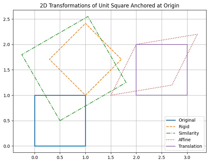
Transformations in homogeneous coordinates
In this section we show common 2D transformations using homogeneous representations.
Rigid Transformation
A rigid transformation preserves lengths and angles — it includes rotation and translation, but no scaling or shearing.
A similarity transformation includes rotation, translation, and uniform scaling. It preserves shape but not necessarily size.
\[
\mathbf{T}_{\text{sim}} =
\begin{bmatrix}
s \cos\theta & -s \sin\theta & t_x \\
s \sin\theta & s \cos\theta & t_y \\
0 & 0 & 1
\end{bmatrix}
\]
Where \(s\) is the scaling factor.
Affine Transformation
Affine transformations include translation, rotation, scaling, shearing, and combinations. They preserve parallelism of lines but not necessarily lengths or angles.