import numpy as np
import matplotlib.pyplot as plt
from skimage import io

np.set_printoptions(precision=2)![]()
Copyright (c) 2021, 2022, Sudeep Sarkar, University of South Florida, Tampa
Scikit-image
scikit-image is a collection of algorithms for image processing. It is available free of charge and free of restriction.
https://scikit-image.org/
https://scikit-image.org/docs/dev/user_guide/getting_started.html
Code: Mount Google drive to access your file structure
You can store your input and output files on your Google drive so that they persist across sessions.
From Canvas, download the zip-file of images we will use in this course into your Google drive. Store them under the directory:
MyDrive/Colab Notebooks/CAP 6415 Computer Vision Online/data/You can do this upload from the web or from your desktop. You can use the desktop version of Google drive and mount it on your laptop to have local access to the gdrive files. See https://www.google.com/drive/download/
Below is the code to mount your Google Drive onto this Colab instance. You will have to do this every time you start Colab as you get a new Colab session with a new file structure. This means that anything you save locally on Colab is lost, and you have to save it in your Google drive to access it across sessions.
## Mount Google drive
from google.colab import drive
drive.mount('/content/drive')
data_dir = '/content/drive/MyDrive/Colab Notebooks/CAP 6415 Computer Vision Online/data/'

!ls "$data_dir"
Mounted at /content/drive
0005_Walking001.xlsx Fig3_4c.jpg left11.jpg
0008_ChaCha001.xlsx hawaii.png left12.jpg
2011_09_26_drive_0048_sync house_1.png lizard.jpg
2011_09_26_drive_0048_sync.zip house_2.png MOT16-08-raw.webm
20211003_082148.jpg house_facade.png mountain_peak_1.png
20211003_082201.jpg IMG_0185.jpg mountain_peak_2.png
apple.jpg IMG_0186.jpg parking_lot_meva_1.png
'Armes 1.png' kellog.jpg parking_lot_meva_2.png
'Armes 2.png' left01.jpg parking_lot_meva_3.png
blog_danforth_monica_mural_panorama.jpg left02.jpg 'Road Signs Kaggle'
blog_monica_mural_brown_white.jpg left03.jpg semper
blog_monica_mural_fish_tree_windows1.jpg left04.jpg 'Superbowl 2021_1.png'
'cats and dogs.jpg' left05.jpg 'Superbowl 2021_2.png'
convenience-store-cereal01.jpg left06.jpg 'Superbowl 2021_3.png'
declaration_of_independence_stone_630.jpg left07.jpg Total-Text-Dataset
Fig3_3a.jpg left08.jpg Wildtrack
Fig3_4a.jpg left09.jpgBasics of images
In the this and next units we will introduce to you how images are represented using arrays and how you can manipulate the value of the arrays to change the image appearance. You will learn through actual code how image thresholding and simple logical operations can be used to separate text in images taken of printed pages. This is something at all text scanning apps do.
Image formation
There is the photometric aspect, and then there is the geometric aspect.
The photometric aspects has to do with the brightness and color of the image, which is a function of the light source, surface characteristics (shiny, glossy, matte), and surface orientation with respect to the camera.
The image is a 2D structure, whereas the world is 3D. We lose a dimension of the world when we capture an image! This dimensional loss leads to artifacts such as parallel lines in the world (think rail lines) that do not appears as parallels in images. We will study these aspects in the following lecture.

The above figure is from the textbook Computer Vision: Algorithms and Applications 2nd Edition Richard Szeliski - (c) 2022 Springer
Code: Read image
- An image is represented in a computer as an array of pixels – a three-dimensional array (row, col, color).
- Color at a pixel is captured by three numbers that represent the number of primary colors - red, blue, green.
'''
Read in an image,
'''
# Load an color image
imfile_name = data_dir+'apple.jpg'

color_img = io.imread(imfile_name)
print ('\n Size of color image array (#row, #col, rgb):', color_img.shape, 'Data type:', color_img.dtype)
print('\n Pixel values at row 200 and col 520: (red, green, blue)\n', color_img[200,520,:])
print('\n Pixel values of a 2 by 2 block\n', color_img[200:202,520:522,:])

# plot the image on screen and other plots
plt.figure(figsize=(15,10))

plt.subplot(1,2,1)
plt.imshow(color_img);

plt.subplot(1,2,2)
plt.imshow(color_img[200:210,520:530,:]);
 Size of color image array (#row, #col, rgb): (612, 612, 3) Data type: uint8

 Pixel values at row 200 and col 520: (red, green, blue)
 [168  45  38]

 Pixel values of a 2 by 2 block
 [[[168  45  38]
  [152  34  24]]

 [[143  20  13]
  [176  58  46]]]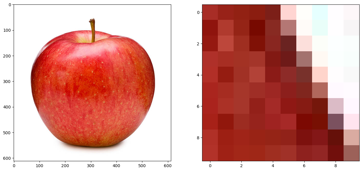
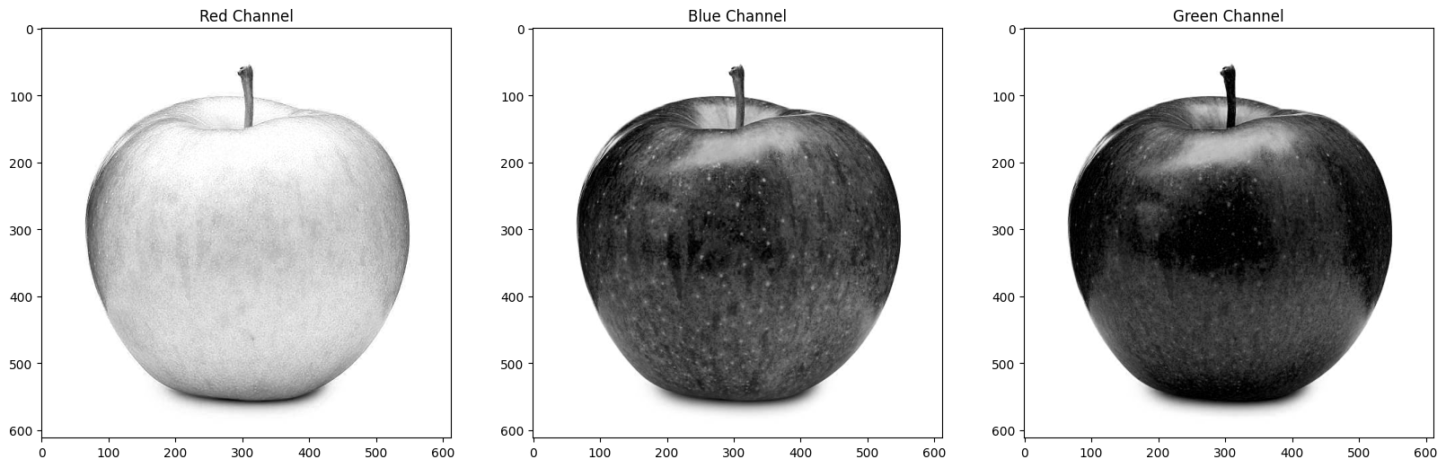
Code: Color channels
# Show the blue, green, red channels

# Example of how to create plots
# using the variable axs for multiple Axes
fig, axs = plt.subplots(1, 3)
fig.set_size_inches (20, 10)

axs[0].imshow(color_img[:,:,0], 'gray');
axs[0].set_title('Red Channel')

axs[1].imshow(color_img[:,:,1], 'gray');
axs[1].set_title('Blue Channel')

axs[2].imshow(color_img[:,:,2], 'gray');
axs[2].set_title('Green Channel');
Code: Gray level image
'''
Gray level image = average of the 3 color channels
'''
gray_img = (color_img[:,:,0].astype(float) + color_img[:,:,1].astype(float) + color_img[:,:,2].astype(float))/3
# What is the "astype" extension doing? Why do we need it?
gray_img = gray_img.astype (np.uint8)

print('\n Size of gray level image:', gray_img.shape, 'Data type:', gray_img.dtype)

fig, axs = plt.subplots(1, 2)
fig.set_size_inches (20, 10)
axs[0].imshow(gray_img, 'gray');
axs[0].set_title('Simply averaged gray image');

# The following combination of RGB better represents what human's perceive as gray level in a color image.
# Y = 0.2125 R + 0.7154 G + 0.0721 B
# You can learn more about color perception at http://poynton.ca/PDFs/ColorFAQ.pdf
#
# Color perception and representation in images is not a simple matter. There are books written on this topic.
# See for example, https://en.wikipedia.org/wiki/Color_vision
#
# RGB is not the best representation.

xyz_gray_img = (0.2125 * color_img[:,:,0].astype(float) + 0.7154 * color_img[:,:,1].astype(float) + 0.0721 * color_img[:,:,2].astype(float))/3
xyz_gray_img = xyz_gray_img.astype (np.uint8)

axs[1].imshow(xyz_gray_img, 'gray');
axs[1].set_title('XYZ-based gray image');
Size of gray level image: (612, 612) Data type: uint8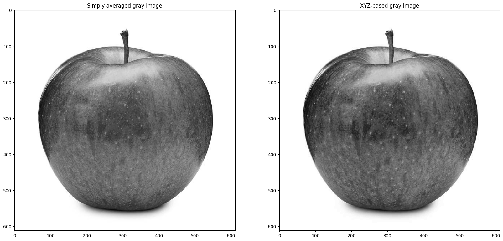
Processing Document Images
imfile_name = data_dir + 'declaration_of_independence_stone_630.jpg'
doi = io.imread(imfile_name)


from skimage import color as change # contains function to change between color spaces

gdoi = change.rgb2gray(doi)
print('Gray level image array: \n', gdoi)

'''
# The rgb2gray function turns rgb image to gray, however, note the range. It is from 0 to 1.
# This mapping of the gray level intensity to the range 0 and 1 is specific to the function
# rgb2gray used here. There might be other image processing packages that keep the range to be
# between 0 and 255. You have to be careful about this aspects of transformation functions,
# i.e. range over which the output values are mapped. Typically, this range is (0, 1) or (0, 255).
'''

fig, axs = plt.subplots(1, 2)
fig.set_size_inches (20, 10)

axs[0].imshow(doi);
axs[0].set_title('Color Image');

axs[1].imshow(gdoi, 'gray');
axs[1].set_title('Gray Image');
Gray level image array:
[[0.91 0.91 0.92 ... 0.9 0.9 0.9 ]
[0.91 0.91 0.9 ... 0.9 0.9 0.9 ]
[0.91 0.91 0.88 ... 0.9 0.9 0.9 ]
...
[0.91 0.91 0.91 ... 0.9 0.9 0.9 ]
[0.91 0.91 0.91 ... 0.9 0.9 0.91]
[0.91 0.91 0.91 ... 0.91 0.91 0.9 ]]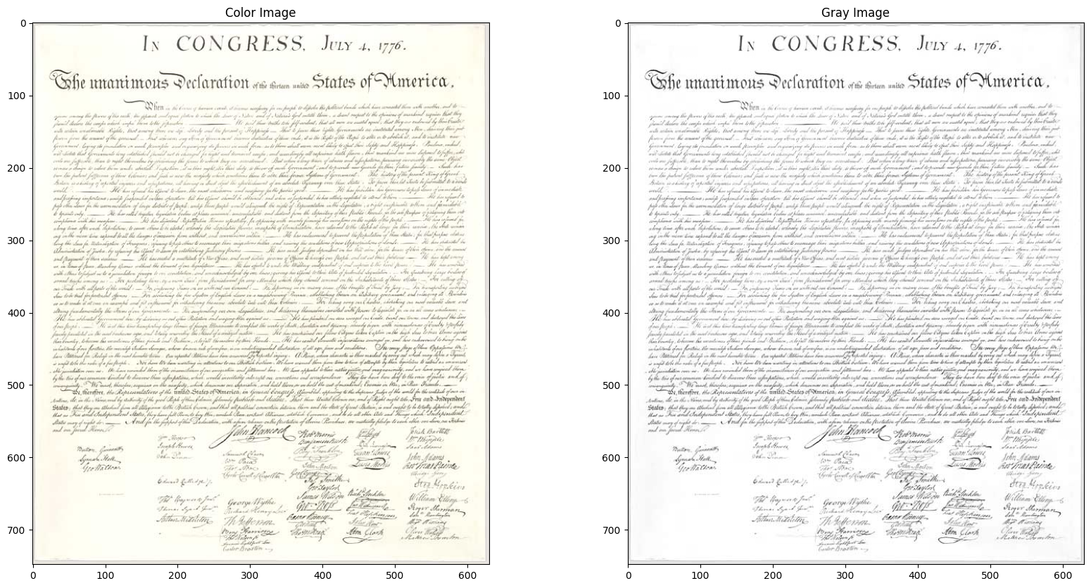
Code: Image Thresholding
fig, axs = plt.subplots(2, 1)
fig.set_size_inches (40, 20)

axs[0].imshow(gdoi[1:200,:], 'gray');
axs[0].set_title('Color image');

'''
Thresholding
'''
bw_doi = np.where( gdoi > 0.8, 0, 1)

print (bw_doi)
axs[1].imshow(bw_doi[1:200,:], 'gray');
axs[1].set_title('Black White image');
[[0 0 0 ... 0 0 0]
[0 0 0 ... 0 0 0]
[0 0 0 ... 0 0 0]
...
[0 0 0 ... 0 0 0]
[0 0 0 ... 0 0 0]
[0 0 0 ... 0 0 0]]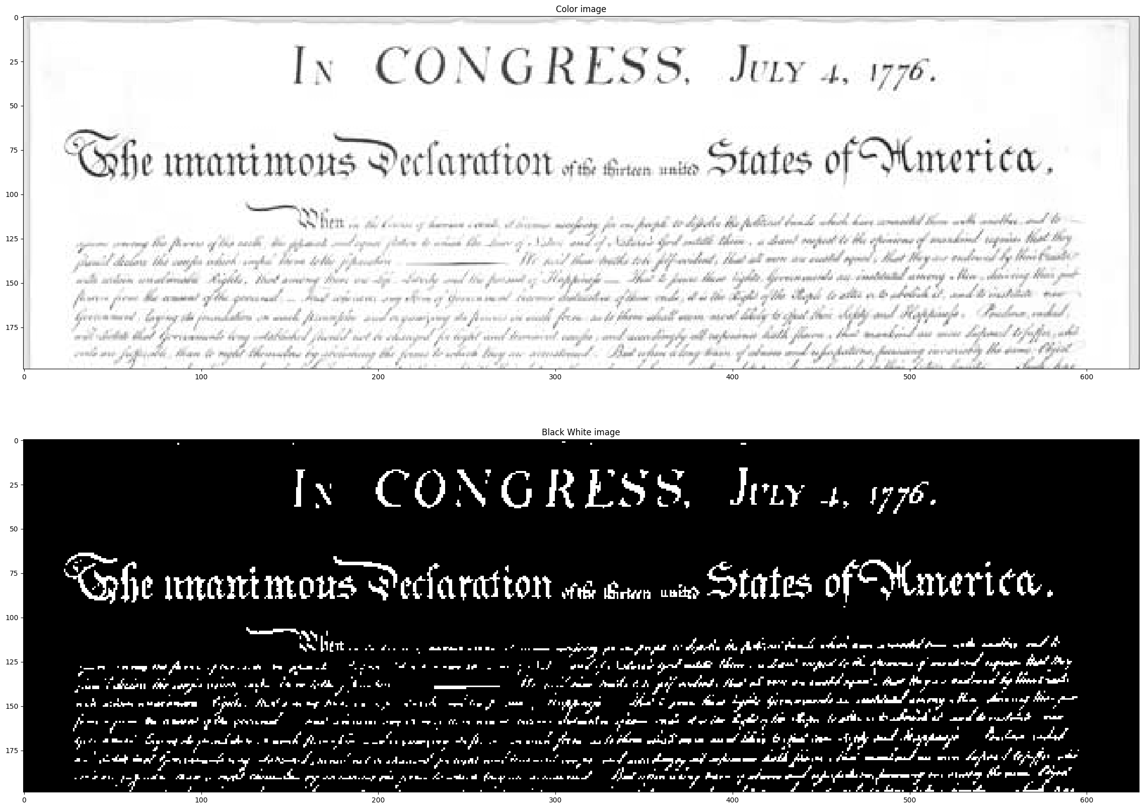
Code: Image histogram
The image histogram is the plot of the pixel count of different values.
ax = plt.hist(doi.ravel(), bins = 100)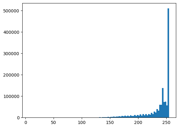
Code: Sum foreground pixels in each row
We plot of the number of pixels in the thresholded image with a value of 255 along each row.
We can use this signal to break up the document into lines.
Idea: Look for the local minima. How would you detect them?
fig, axs = plt.subplots(2, 1)
fig.set_size_inches (20, 20)

num_255_row = np.sum(bw_doi, axis=1)

axs[0].plot(num_255_row[1:200]);
axs[0].set_title('Number of pixels with 255 along each row');
axs[1].imshow(bw_doi[1:200,:], 'gray');
axs[1].set_title('Black White image');

minima_locations = np.zeros(num_255_row.shape)
for i in range(1, 200) :
    if ((num_255_row[i] < num_255_row[i-1]) and (num_255_row[i] < num_255_row[i+1])):
       # logic to detect minima at [i], which should be lower than at i+1 and i-1

        if (num_255_row[i] < 25) : # the minimum should have a low value, less than 25 white pixels

            axs[0].plot (i-1, num_255_row[i], 'r*')
# Why are we using i-1 to mark the minima location rather than i in the plot?
# Ans: The plot starts at horizontal axis = 1 not 0.
            axs[1].plot(np.array([0, bw_doi.shape[1]]), np.array([i, i]), 'y')
            minima_locations[i] = 1
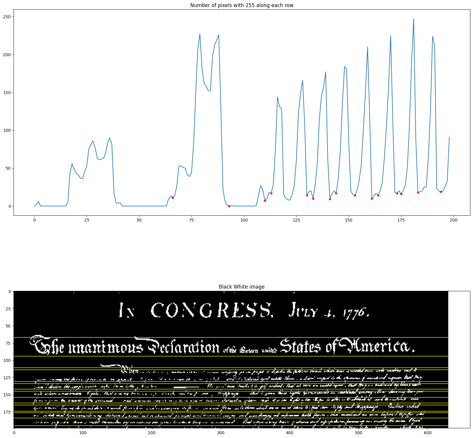
Homework: line segmentation in documents
Notice that in the output above, the top and bottom line for the text “In Congress July 4, 1976” is not detected. Can you find other boundary lines that are missing?
Fix the logic in line 13 to detect these missing lines.
Submit as instructed on Canvas.
Use Case: Turn Scanned Document into Text
Text detection and recognition in scanned documents have many uses, e.g., digital library initiatives. There is a need to create searchable texts from scanned old books and manuscripts, most of which are now hidden from the current generation, who rely on just digitized information.
Some advanced camera-based document scanning apps on your phone allow you to create an editable text version of the imaged pages. These apps are essentially performing text detection and recognition.
What you have seen is just the first step towards building a complete algorithm – the line detection step. After detecting each line, we again break each line into words using the gap signatures. Once each word on the page is outlined, we send the sub-image to an Optical Character Recognition (OCR) algorithm to classify it into a word-text representation.
Here are examples of available software that you can play with
https://cloud.google.com/vision/docs/ocr
- In general, creating editable text from scanned typed or printed documents is more straightforward than turning scanned handwritten documents into text.