import math
import torch
import torch.nn as nn
import torch.nn.functional as F

torch.manual_seed(0)


def gaussian_nll(y, mu, log_var):
    """
    Per-sample Gaussian negative log-likelihood (up to additive constant):
        0.5 * [ log σ^2(x) + (y - μ(x))^2 / σ^2(x) ]
    y, mu, log_var: (B,)
    """
return 0.5 * (log_var + (y - mu) ** 2 * torch.exp(-log_var))SGD Regression with Gaussian NLL: Mean & Variance (Aleatoric) Estimation
This notebook replaces MSE with a Gaussian negative log-likelihood (NLL) so that SGD jointly learns the predictive mean ((x)) and variance (^2(x)). It includes both heteroscedastic (input-dependent variance) and an optional homoscedastic (single variance) variant, along with visualization of 95% prediction intervals.
Gaussian NLL utilities
Data
Uses existing x_train, y_train if already defined in the kernel; otherwise generates a sinusoidal dataset with heteroscedastic noise for a meaningful demo.
import numpy as np


def _to_tensor(x):
    x = torch.as_tensor(x, dtype=torch.float32)
    return x


globals_exist = all(name in globals() for name in ["x_train", "y_train"])
if not globals_exist:
    n_train = 256
    n_test = 400
    x = np.random.uniform(-3.0, 3.0, size=(n_train, 1)).astype(np.float32)
    # heteroscedastic noise: sigma grows with |x|
    sigma = 0.15 + 0.25 * (np.abs(x).squeeze())
    y = np.sin(1.3 * x).squeeze() + np.random.normal(0.0, sigma)
    x_train = _to_tensor(x)
    y_train = _to_tensor(y)

    # grid for visualization
    xs = np.linspace(-3.5, 3.5, n_test).reshape(-1, 1).astype(np.float32)
    x_test = _to_tensor(xs)
else:
    if "x_test" not in globals():
        x_min = float(torch.min(x_train))
        x_max = float(torch.max(x_train))
        xs = (
            np.linspace(x_min - 0.25 * (x_max - x_min), x_max + 0.25 * (x_max - x_min), 400)
            .reshape(-1, 1)
            .astype(np.float32)
        )
        x_test = _to_tensor(xs)

x_train.shape, y_train.shape, x_test.shape
(torch.Size([256, 1]), torch.Size([256]), torch.Size([400, 1]))Heteroscedastic Regressor: predicts μ(x) and log σ²(x)
class MeanVarRegressor(nn.Module):
    def __init__(self, in_dim=1, hidden=128):
        super().__init__()
        self.shared = nn.Sequential(
            nn.Linear(in_dim, hidden),
            nn.ReLU(),
            nn.Linear(hidden, hidden),
            nn.ReLU(),
        )
        self.mu_head = nn.Linear(hidden, 1)
        self.logvar_head = nn.Linear(hidden, 1)

        # Initialize logvar head bias to a small negative value
        nn.init.constant_(self.logvar_head.bias, -1.0)

    def forward(self, x):
        h = self.shared(x)
        mu = self.mu_head(h).squeeze(-1)  # (B,)
        # Ensure positive variance via softplus, then take log
        log_var = torch.log(F.softplus(self.logvar_head(h).squeeze(-1)) + 1e-6)
        return mu, log_var


model = MeanVarRegressor(in_dim=x_train.shape[1], hidden=128)
model
MeanVarRegressor(
(shared): Sequential(
(0): Linear(in_features=1, out_features=128, bias=True)
(1): ReLU()
(2): Linear(in_features=128, out_features=128, bias=True)
(3): ReLU()
)
(mu_head): Linear(in_features=128, out_features=1, bias=True)
(logvar_head): Linear(in_features=128, out_features=1, bias=True)
)Train with SGD on Gaussian NLL
from torch.utils.data import TensorDataset, DataLoader

batch_size = 64
epochs = 800
lr = 5e-3
weight_decay = 1e-4  # curbs variance inflation

ds = TensorDataset(x_train, y_train)
dl = DataLoader(ds, batch_size=batch_size, shuffle=True)

opt = torch.optim.SGD(model.parameters(), lr=lr, momentum=0.9, weight_decay=weight_decay)

model.train()
for epoch in range(1, epochs + 1):
    running = 0.0
    for xb, yb in dl:
        mu, log_var = model(xb)
        loss = gaussian_nll(yb, mu, log_var).mean()
        opt.zero_grad()
        loss.backward()
        opt.step()
        running += loss.item() * xb.size(0)
    if epoch % 100 == 0:
        print(f"epoch {epoch:4d} | nll: {running / len(ds):.4f}")
epoch 100 | nll: -0.2359
epoch 200 | nll: -0.2312
epoch 300 | nll: -0.2350
epoch 400 | nll: -0.2295
epoch 500 | nll: -0.2332
epoch 600 | nll: -0.2457
epoch 700 | nll: -0.2408
epoch 800 | nll: -0.2491Predictive mean and 95% intervals
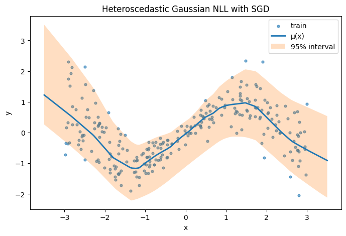
model.eval()
with torch.no_grad():
    mu_pred, log_var_pred = model(x_test)
    sigma_pred = torch.exp(0.5 * log_var_pred)
    lo = mu_pred - 1.96 * sigma_pred
    hi = mu_pred + 1.96 * sigma_pred

mu_pred.shape, sigma_pred.shape
(torch.Size([400]), torch.Size([400]))Plot
import matplotlib.pyplot as plt

plt.figure(figsize=(8, 5))
plt.scatter(x_train.numpy().squeeze(), y_train.numpy().squeeze(), s=12, alpha=0.6, label="train")
plt.plot(x_test.numpy().squeeze(), mu_pred.numpy().squeeze(), linewidth=2, label="μ(x)")
plt.fill_between(
    x_test.numpy().squeeze(), lo.numpy().squeeze(), hi.numpy().squeeze(), alpha=0.25, label="95% interval"
)
plt.legend()
plt.title("Heteroscedastic Gaussian NLL with SGD")
plt.xlabel("x")
plt.ylabel("y")
plt.show()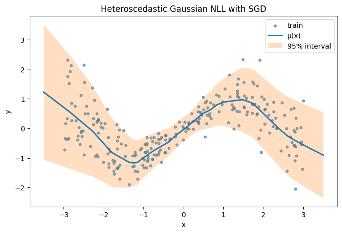
Optional: Homoscedastic Variant (single learned σ²)
class MeanOnlyRegressor(nn.Module):
    def __init__(self, in_dim=1, hidden=128):
        super().__init__()
        self.net = nn.Sequential(
            nn.Linear(in_dim, hidden), nn.ReLU(), nn.Linear(hidden, hidden), nn.ReLU(), nn.Linear(hidden, 1)
        )
        self.log_var = nn.Parameter(torch.tensor(0.0))

    def forward(self, x):
        mu = self.net(x).squeeze(-1)
        log_var = self.log_var.expand_as(mu)
        return mu, log_var


# Example quick train:
model_h = MeanOnlyRegressor(in_dim=x_train.shape[1], hidden=128)
opt_h = torch.optim.SGD(model_h.parameters(), lr=5e-3, momentum=0.9, weight_decay=1e-4)

for epoch in range(300):
    mu, log_var = model_h(x_train)
    loss = gaussian_nll(y_train, mu, log_var).mean()
    opt_h.zero_grad()
    loss.backward()
    opt_h.step()

with torch.no_grad():
    mu_h, logv_h = model_h(x_test)
    sig_h = torch.exp(0.5 * logv_h)
    lo_h, hi_h = mu_h - 1.96 * sig_h, mu_h + 1.96 * sig_h
import matplotlib.pyplot as plt

plt.figure(figsize=(8, 5))
plt.scatter(x_train.numpy().squeeze(), y_train.numpy().squeeze(), s=12, alpha=0.6, label="train")
plt.plot(x_test.numpy().squeeze(), mu_pred.numpy().squeeze(), linewidth=2, label="μ(x)")
plt.fill_between(
    x_test.numpy().squeeze(), lo_h.numpy().squeeze(), hi.numpy().squeeze(), alpha=0.25, label="95% interval"
)
plt.legend()
plt.title("Heteroscedastic Gaussian NLL with SGD")
plt.xlabel("x")
plt.ylabel("y")
plt.show()