Why whitening helps
The input
It is instructive to see the training process as a control system.

The system takes input \(\mathbf x\) and produces a loss that is used to update the parameters \(\mathbf w\) for each of the layers based on a estimate of how much the loss \(L\) changed for that input. There are multiple concepts in this sentence that is worth highlighting. First lets repeat the SGD equation below as it will used to drive the discussion.
\[\mathbf w_{k+1} = \mathbf w_k - \eta \nabla_{\mathbf w} L(\mathbf w_k)\]
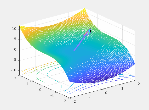
It is enough to discuss the limiting case with just two parameters to visualize the loss as shown below. This is obviously a 3D plot with x and y axes on parameters and the z axis assigned to loss.
Recall that back-propagation starts from where forward propagation ends, so the batched input is the driving force of the learning process and the noisy negative gradient of the loss with respect to weights is a search direction of where to look for a possible reductions of that loss. The control system’s optimizer feedbacks the parameter updates every mini-batch hopping that successive updates will converge to some good local minimum.
As described in this paper, networks learn the fastest from the most unexpected examples. If this rings the bells of Shannon’s value of information we saw in the entropy section, it should. One way to maximize the unexpectedness is in each iteration to choose input examples that belong to different classes expecting that they will also contain significantly different information. In practice we can approximate this with a permutation over the examples (epochs).
So what we do at the input is important and as you can see from even this very limiting case, the loss surface \(L(\mathbf w) = L(\hat y, y) = L(\sigma(w^Tx), y)\) over all possible weights is very much changing at each iteration (mini-batch). So if we are stuck in a bad local minima at iteration \(k\) chances are in the next iteration \(k+1\) we wont as the loss surface may not have a local minima there. In summary permuting the inputs brings a very positive net benefit to training as we break correlations in time.
The whitening / decorrelation process
Whitening is a more advanced form of normalization that aims to remove correlations between input features and standardize the input distribution. It involves transforming the input data so that it has a mean of 0, a variance of 1, and a covariance matrix that is the identity matrix (i.e., the features become uncorrelated).
Whitening is rarely used in practice for image data in modern deep learning frameworks, but I can explain how it would be done for the MNIST dataset if it were applied.
Steps to Apply Whitening to MNIST:
- Reshape the Input:
- Each image in MNIST is 28x28 pixels, which gives you 784 pixels (features) for each image.
- Flatten each image into a 1D vector of 784 elements. So, for a dataset of (N) images, the data matrix (X) will have shape (N ), where each row is an image.
- Center the Data (Zero Mean):
- Subtract the mean of each feature (pixel) across all images so that each feature has a mean of 0. This is done column-wise (for each feature). [ X_{} = X - ] where ( ) is the mean vector of shape ( 784 ), containing the mean pixel intensity for each feature across all ( N ) images.
- Compute the Covariance Matrix:
- Compute the covariance matrix of the centered data. The covariance matrix will have a shape of ( 784 ), where each element ((i, j)) represents the covariance between the (i)-th and (j)-th pixel across all images. [ = X_{}^T X_{} ] where ( ) is the ( 784 ) covariance matrix.
- Eigenvalue Decomposition or Singular Value Decomposition (SVD):
- Perform eigenvalue decomposition or SVD on the covariance matrix ( ). This step will give you the eigenvalues and eigenvectors (principal components) of the covariance matrix. [ = U U^T ] where:
- ( U ) is a matrix of eigenvectors (shape ( 784 )).
- ( ) is a diagonal matrix of eigenvalues (shape ( 784 )).
- Whitening Transformation:
- Now, apply the whitening transformation. This transformation uses the eigenvectors and eigenvalues of the covariance matrix to scale and rotate the data such that the covariance matrix of the transformed data becomes the identity matrix. The transformation is given by: [ X_{} = X_{} U ^{-} U^T ]
- Here, ( ^{-} ) is the inverse square root of the eigenvalue matrix, which scales the data so that the variance of each component is 1.
- The result is that the features (pixels) of ( X_{} ) are uncorrelated and have unit variance.
- Reshape Back:
- After whitening, reshape the 1D feature vectors back into the original image shape (28x28 pixels) for each image if needed.
Python Implementation of Whitening for MNIST
Here’s an example using NumPy for whitening the MNIST dataset:
import numpy as np
from sklearn.datasets import fetch_openml

# Step 1: Load MNIST dataset
mnist = fetch_openml('mnist_784')
X = mnist.data  # Shape: (70000, 784)

# Step 2: Center the data (subtract mean)
mean = np.mean(X, axis=0)
X_centered = X - mean

# Step 3: Compute covariance matrix
cov_matrix = np.cov(X_centered, rowvar=False)

# Step 4: Eigenvalue decomposition (or SVD)
eigvals, eigvecs = np.linalg.eigh(cov_matrix)

# Step 5: Whitening transformation
# Eigenvalue scaling (Lambda^(-1/2))
eigvals_inv_sqrt = np.diag(1.0 / np.sqrt(eigvals + 1e-5))  # Add small value to avoid division by zero
X_whitened = X_centered.dot(eigvecs).dot(eigvals_inv_sqrt).dot(eigvecs.T)

print("Whitened data shape:", X_whitened.shape)
Explanation of the Code:
- Centering: The data is centered by subtracting the mean of each feature (pixel).
- Covariance Matrix: The covariance matrix of the centered data is computed.
- Eigenvalue Decomposition: Eigenvalue decomposition is used to get the eigenvalues and eigenvectors.
- Whitening Transformation: The data is whitened by multiplying the centered data by the eigenvectors and scaling by the inverse square root of the eigenvalues.
Why Whitening is Rarely Used in Practice:
- Computational Complexity: Whitening involves calculating the covariance matrix and performing eigenvalue decomposition or SVD, which can be computationally expensive, especially for large datasets.
- Batch Normalization: In deep learning, batch normalization is a much simpler and more effective technique to stabilize training and normalize the activations of each layer. This method has largely replaced the need for whitening in neural network training.
Summary:
- Whitening for MNIST involves zero-centering the data, computing the covariance matrix, and applying a transformation based on the eigenvalue decomposition of the covariance matrix to decorrelate the features.
- Although theoretically useful, whitening is computationally expensive and has largely been replaced by more efficient normalization techniques like batch normalization in modern deep learning practices.