Bayesian Inference
The Bayes Rule
 Thomas Bayes (1701-1761)
The Bayesian theorem is the cornerstone of probabilistic modeling and ultimately governs what models we can construct inside the learning algorithm. If \(\mathbf{w}\) denotes the unknown parameters, \(\mathtt{data}\) denotes the dataset and \(\mathcal{H}\) denotes the hypothesis set that we met in the learning problem chapter.
\[ p(\mathbf{w} | \mathtt{data}, \mathcal{H}) = \frac{P( \mathtt{data} | \mathbf{w}, \mathcal{H}) P(\mathbf{w} | \mathcal{H}) }{ P( \mathtt{data} | \mathcal{H})} \]
The Bayesian framework allows the introduction of priors \(p(\mathbf w | \mathcal{H})\) from a wide variety of sources: experts, other data, past posteriors, etc. It allows us to calculate the posterior distribution from the likelihood function and this prior subject to a normalizing constant.
We will call belief the internal to the agent posterior probability estimate of a random variable as calculated via the Bayes rule.
For example,a medical patient is exhibiting symptoms x, y and z. There are a number of diseases that could be causing all of them, but only a single disease is present. A doctor (the expert) has a belief about the underlying disease, but a second doctor may have a slightly different belief.
Bayesian approach vs Maximum Likelihood
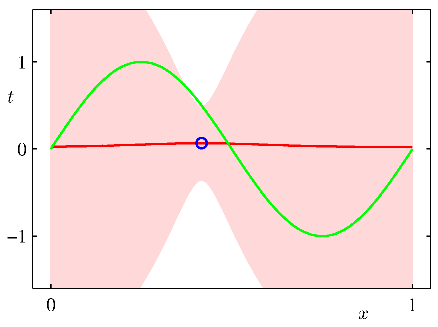
In the Maximum Likelihood Estimation section we have seen a simple supervised learning problem that is specified via a joint distribution \(\hat{p}_{data}(\mathbf x, y)\) and are asked to fit the model parameterized by the weights \(\mathbf w\) using maximum likelihood. Its important to view pictorially perhaps the most important effect of Bayesian thinking in the regression setting:
The \(\mathbf{w}\) in MLE is a point estimate \(\mathbf{w}_{MLE}\) and we are plugging this estimate in the predictive distribution to make predictions \(\hat y\) for data we havent seen before.
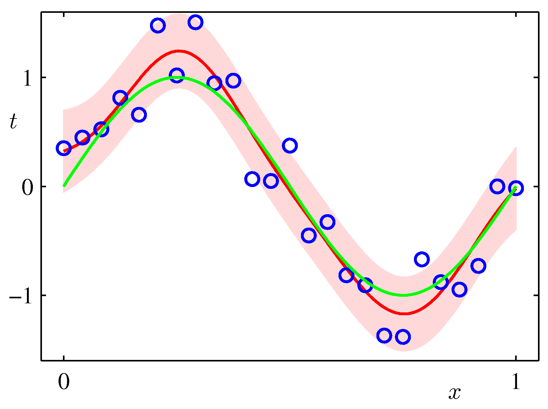
In the Bayesian setting on the other hand we use a full distribution over \(\mathbf w\). We predict by integrating over the posterior of \(\mathbf{w}\) (i.e. given the data) and therefore considering organically the uncertainty of the posterior of \(\mathbf{w}\) in our predictions. As such it can capture the effects of sparse data producing more uncertainty via its covariance in areas where there are no data as shown in the following example which is exactly the same sinusoidal dataset fit with Bayesian updates and Gaussian basis functions.

ML frameworks have been enhanced recently to deal with Bayesian approaches and approximations that make such approaches feasible for both classical and deep learning. TF.Probability and PyTorch Pyro are examples of such enhancements.
Before diving into the posterior update in regression problems its instructive to go over the Bayesian coin tossing notebook that shows a simpler experiment.