The Probabilistic Graphical Model is a representation that is extensively used in probabilistic reasoning. Lets consider the simplest possible example of a graphical model and see how it connects to concepts we have seen before. Any joint distribution \(p(\mathbf x, y)\) can be decomposed using the product rule (we drop the data qualifier)

\[p(\mathbf x, y) = p(\mathbf x) p(y|\mathbf x)\]

and such distribution can be represented via the simple PGM graph (a) below.

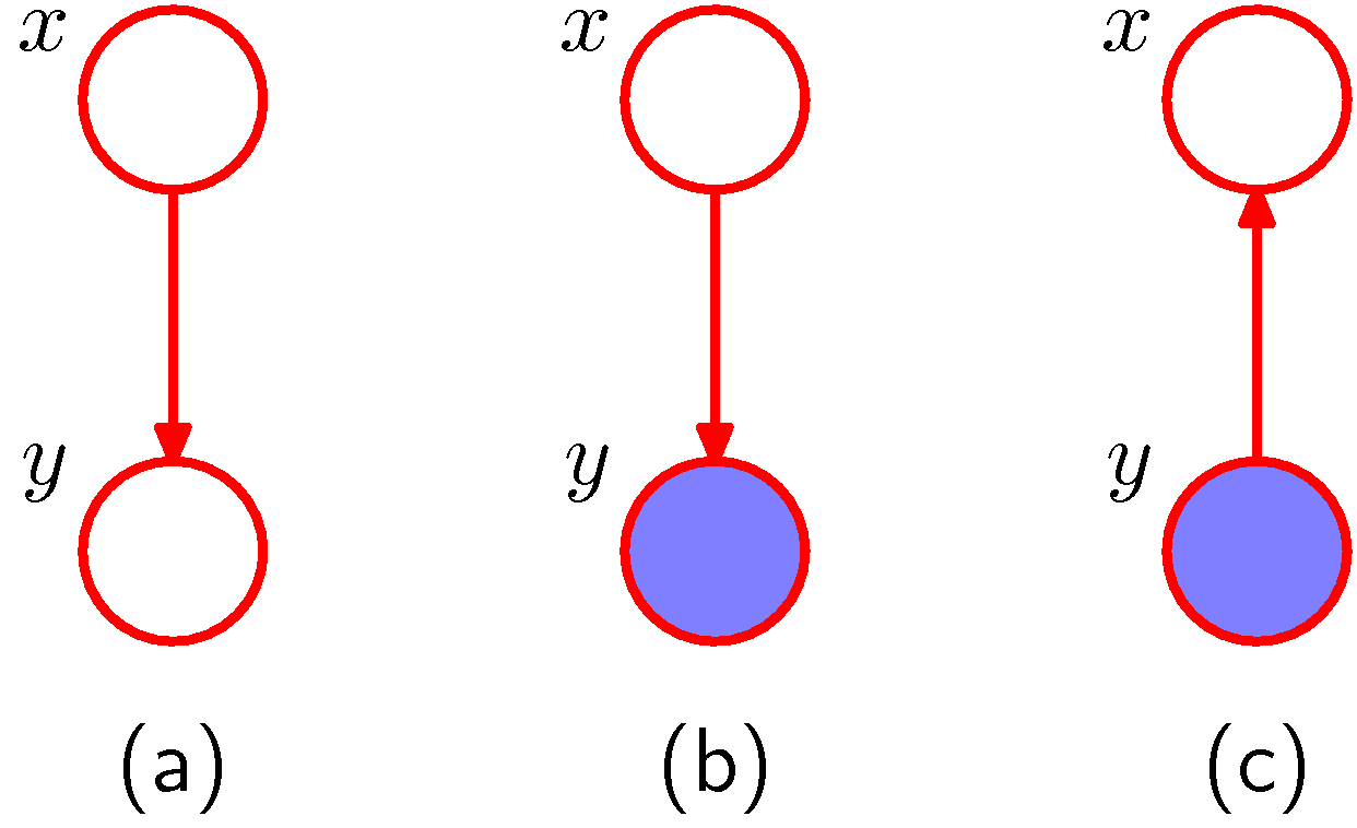
Simplest possible PGM example

We introduce now a graphical notation where we shade, nodes that we consider observed. Let us know assume that we observe \(y\) as shown in (b). We can view the marginal \(p(\mathbf x)\) as a prior over \(x\) and and we can infer the posterior distribution using the Bayes rule

\[p(x|y) = \frac{p(y|x)p(x)}{p(y)}\]

where using the sum rule we know \(p(y) = \sum_{x'} p(y|x') p(x')\). This is a very innocent but very powerful concept.

Bayesian vs Maximum Likelihood

In the linear regression section we have seen a simple supervised learning problem that is specified via a joint distribution \(\hat{p}_{data}(\mathbf x, y)\) and are asked to fit the model parameterized by the weights \(\mathbf w\) using ML. Its important to view pictorially perhaps the most important effect of Bayesian update:

• In ML the \(\mathbf{w}\) is treated as a known quantity with an estimate \(\hat{\mathbf{w}}\) that has a mean and variance resulting from the distribution of \(y\).

• In the Bayesian setting, we are integrating over the distribution of \(\mathbf{w}\) given the data i.e. we are not making a point estimate of \(\mathbf{w}\) but we marginalize out \(\mathbf{w}\). \[p(\mathbf{w}|y) = \frac{p(y|\mathbf{w}) p(\mathbf{w})}{\int p(y|\mathbf{w}) p(\mathbf{w}) d\mathbf{w}}\]

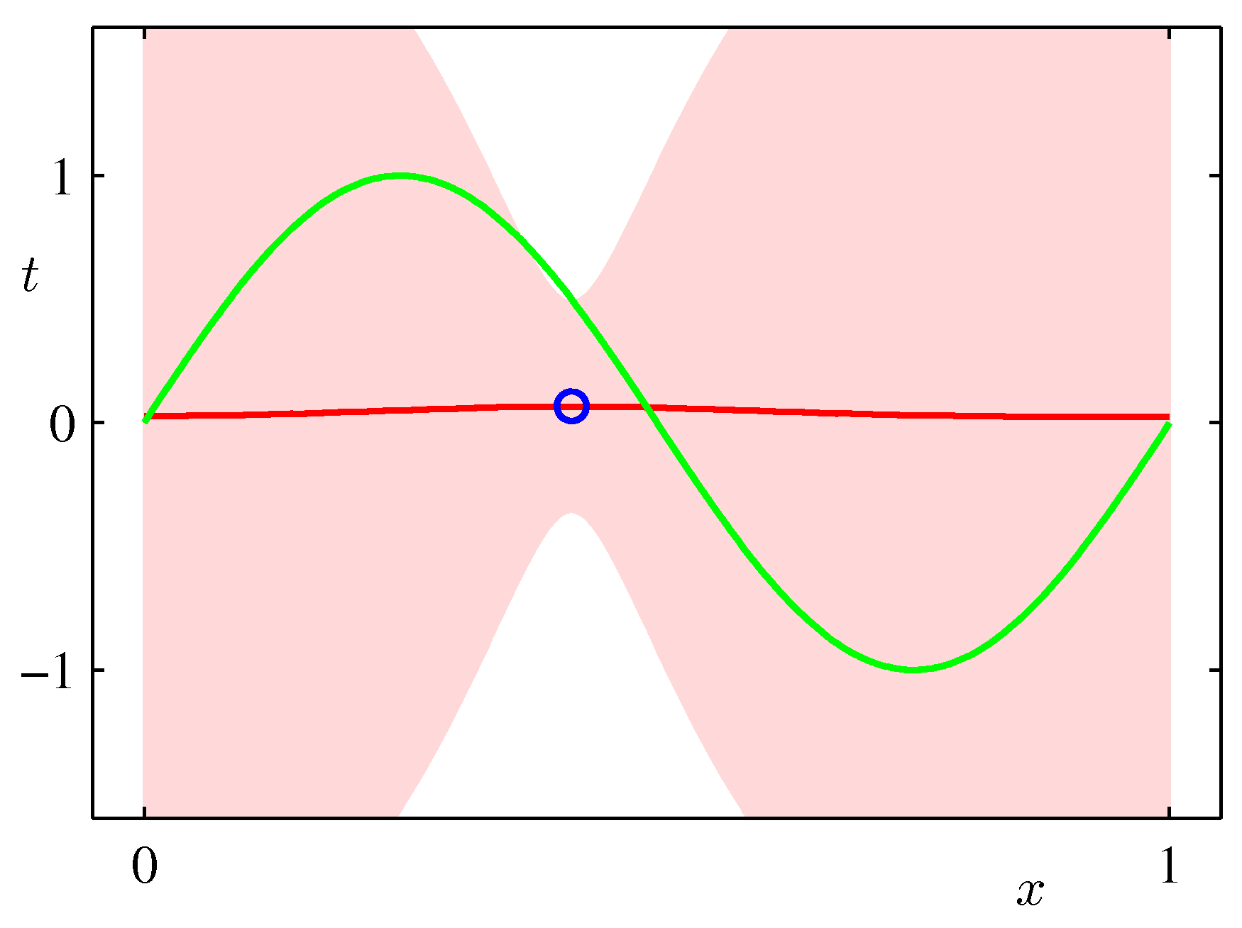
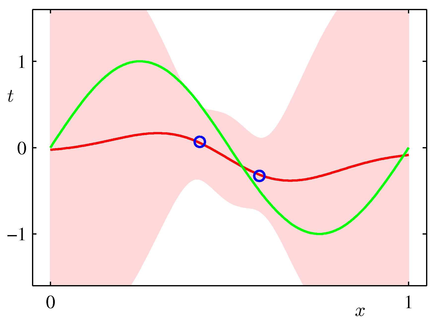
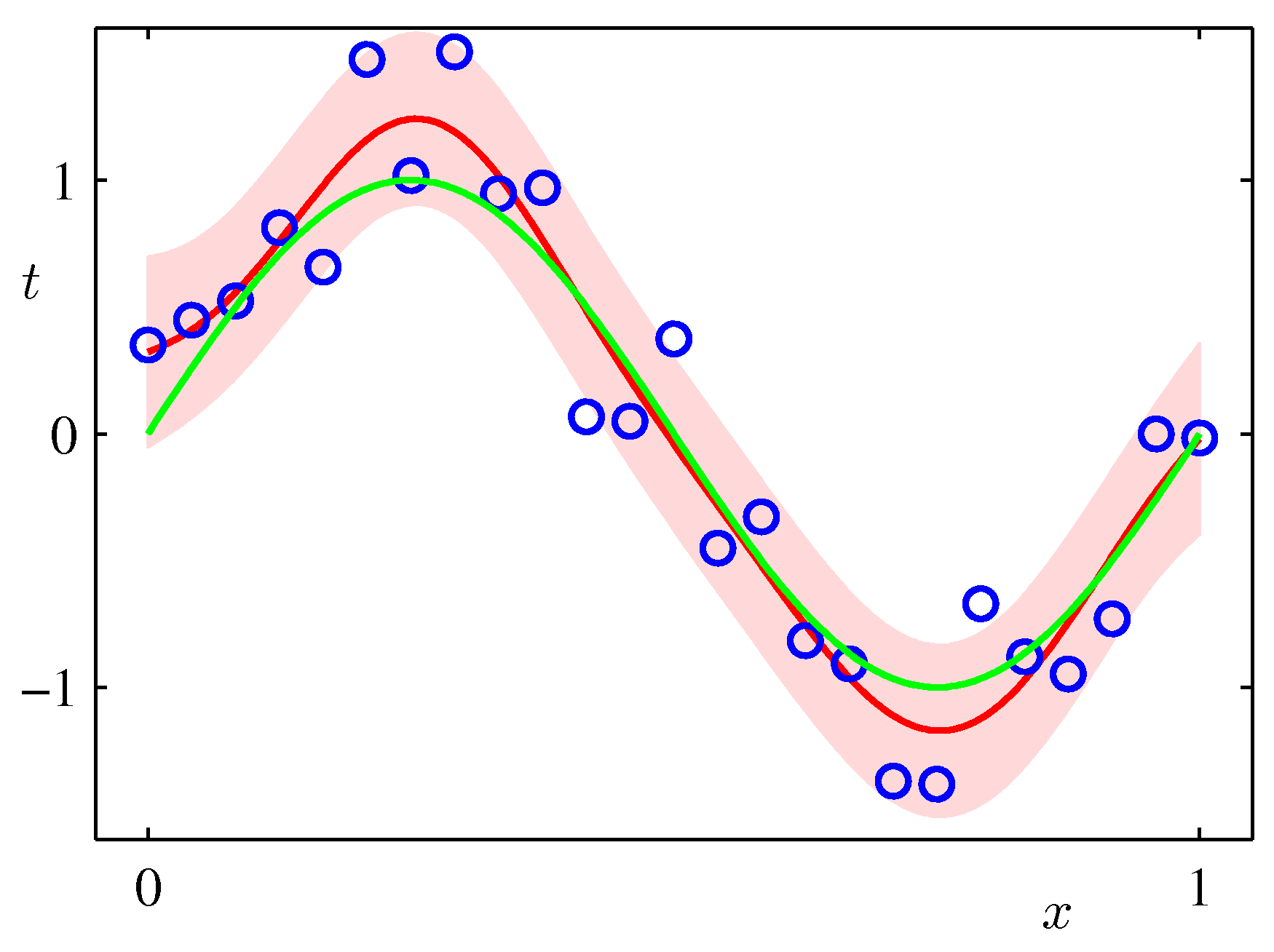
  • We get at the end a posterior (predictive) distribution rather than a point estimate. As such it can capture the effects of sparse data producing more uncertainty via its covariance in areas where there are no data as shown in the following example which is exactly the same sinusoidal dataset fit with Bayesian updates and Gaussian basis functions.

ML frameworks have been enhanced recently to deal with Bayesian approaches and approximations that make such approaches feasible for both classical and deep learning. TF.Probability and PyTorch Pyro are examples of such enhancements.

Bayesian update for discrete problems

HINT: This example is deeper than coin-flipping.