Logistic Regression with SGD on a Gaussian GMM Dataset + PCA

Objective. Generate a synthetic Gaussian Mixture Model (GMM) binary classification dataset where only a low‑dimensional subspace is informative and the remaining dimensions are noisy.
Train logistic regression with SGD in PyTorch with and without PCA, and compare performance.

What students should learn - How redundant/noisy features degrade a linear classifier trained with SGD. - How PCA (unsupervised) can improve performance by denoising and reducing dimensionality. - How to visualize explained variance and decision boundaries in the top PCs.

Setup

import math
import numpy as np
import torch
import torch.nn as nn
from torch.utils.data import TensorDataset, DataLoader
import matplotlib.pyplot as plt

torch.manual_seed(7)
np.random.seed(7)

device = "cpu"


def train_test_split(X, y, test_size=0.3, shuffle=True, seed=0):
    n = X.shape[0]
    idx = np.arange(n)
    if shuffle:
        rng = np.random.default_rng(seed)
        rng.shuffle(idx)
    n_test = int(round(test_size * n))
    test_idx = idx[:n_test]
    train_idx = idx[n_test:]
    return X[train_idx], X[test_idx], y[train_idx], y[test_idx]


def standardize_fit(X):
    mu = X.mean(axis=0, keepdims=True)
    std = X.std(axis=0, keepdims=True) + 1e-8
    return mu, std


def standardize_transform(X, mu, std):
    return (X - mu) / std


def auc_roc(scores, labels):
    scores = np.asarray(scores).ravel()
    labels = np.asarray(labels).astype(int).ravel()
    order = np.argsort(-scores, kind="mergesort")
    y = labels[order]
    P = y.sum()
    N = len(y) - P
    if P == 0 or N == 0:
        return float("nan")
    tps = np.cumsum(y)
    fps = np.cumsum(1 - y)
    tpr = tps / P
    fpr = fps / N
    return float(np.trapz(tpr, fpr))

Generate a GMM dataset (binary) with noisy dimensions

def make_gmm_binary(n_per_class=1000, d_total=20, d_informative=2, class_sep=2.5, noise_std=1.0, seed=0):
    rng = np.random.default_rng(seed)

    sep = class_sep
    mus0 = np.array([[-sep, 0.0], [0.0, -sep]])
    mus1 = np.array([[sep, 0.0], [0.0, sep]])
    cov_inf = np.array([[1.0, 0.3], [0.3, 1.0]])

    def sample_class(mus, n):
        z = rng.integers(0, len(mus), size=n)
        X2 = np.stack([rng.multivariate_normal(mus[k], cov_inf) for k in z], axis=0)
        return X2

    X0_inf = sample_class(mus0, n_per_class)
    X1_inf = sample_class(mus1, n_per_class)

    d_noise = max(0, d_total - d_informative)
    if d_noise > 0:
        X0_noise = rng.normal(0.0, noise_std, size=(n_per_class, d_noise))
        X1_noise = rng.normal(0.0, noise_std, size=(n_per_class, d_noise))
        X0 = np.concatenate([X0_inf, X0_noise], axis=1)
        X1 = np.concatenate([X1_inf, X1_noise], axis=1)
    else:
        X0 = X0_inf
        X1 = X1_inf

    X = np.vstack([X0, X1]).astype(np.float32)
    y = np.concatenate([np.zeros(n_per_class), np.ones(n_per_class)]).astype(np.int64)

    Q, _ = np.linalg.qr(rng.normal(size=(d_total, d_total)))
    X = (X @ Q).astype(np.float32)

    return X, y

# X, y = make_gmm_binary(n_per_class=1200, d_total=20, d_informative=2, class_sep=2.5, noise_std=1.5, seed=42)
X, y = make_gmm_binary(n_per_class=200, d_total=20, d_informative=2, class_sep=2.5, noise_std=1.0, seed=42)

X_train, X_test, y_train, y_test = train_test_split(X, y, test_size=0.3, shuffle=True, seed=123)
mu, std = standardize_fit(X_train)
Xtr = standardize_transform(X_train, mu, std)
Xte = standardize_transform(X_test, mu, std)

X.shape, Xtr.shape, Xte.shape, y_train.shape, y_test.shape

((400, 20), (280, 20), (120, 20), (280,), (120,))

PCA (Torch SVD)

def pca_fit_torch(X_np):
    Xc = X_np - X_np.mean(axis=0, keepdims=True)
    Xc_t = torch.from_numpy(Xc)
    U, S, Vh = torch.linalg.svd(Xc_t, full_matrices=False)
    n = X_np.shape[0]
    ev = (S**2) / (n - 1)
    evr = ev / ev.sum()
    components = Vh.numpy()
    return components, evr.numpy()


def pca_transform(X_np, components, k):
    Xc = X_np - X_np.mean(axis=0, keepdims=True)
    W = components[:k].T
    return (Xc @ W).astype(np.float32)


components, evr = pca_fit_torch(Xtr.copy())
explained = np.cumsum(evr)
k95 = int(np.searchsorted(explained, 0.95) + 1)
k_fixed = 2

print("Explained variance ratio (first 10):", evr[:10])
print("k@95% =", k95)

Explained variance ratio (first 10): [0.14723612 0.12738939 0.06149405 0.05959329 0.05904397 0.05309147
 0.05024018 0.04745107 0.04639223 0.04420933]
k@95% = 18

Plot: cumulative explained variance

plt.figure(figsize=(6, 4))
plt.plot(np.arange(1, len(evr) + 1), np.cumsum(evr), marker="o")
plt.xlabel("number of PCs")
plt.ylabel("cumulative explained variance")
plt.title("PCA cumulative explained variance on training set")
plt.show()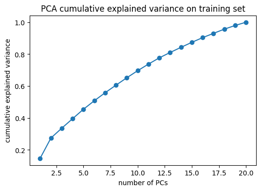

Logistic regression (PyTorch, SGD)

class LogisticReg(nn.Module):
    def __init__(self, in_dim):
        super().__init__()
        self.lin = nn.Linear(in_dim, 1)

    def forward(self, x):
        return self.lin(x).squeeze(-1)


def auc_roc(scores, labels):
    scores = np.asarray(scores).ravel()
    labels = np.asarray(labels).astype(int).ravel()
    order = np.argsort(-scores, kind="mergesort")
    y = labels[order]
    P = y.sum()
    N = len(y) - P
    if P == 0 or N == 0:
        return float("nan")
    tps = np.cumsum(y)
    fps = np.cumsum(1 - y)
    tpr = tps / P
    fpr = fps / N
    return float(np.trapz(tpr, fpr))


def train_logreg_sgd(Xtr_np, ytr_np, Xte_np, yte_np, lr=5e-3, epochs=300, batch_size=128, l2=1e-4):
    Xtr_t = torch.from_numpy(Xtr_np.astype(np.float32))
    ytr_t = torch.from_numpy(ytr_np.astype(np.float32))
    Xte_t = torch.from_numpy(Xte_np.astype(np.float32))
    yte_t = torch.from_numpy(yte_np.astype(np.float32))

    model = LogisticReg(in_dim=Xtr_t.shape[1])
    opt = torch.optim.SGD(model.parameters(), lr=lr, momentum=0.9, weight_decay=l2)
    loss_fn = nn.BCEWithLogitsLoss()

    ds = TensorDataset(Xtr_t, ytr_t)
    dl = DataLoader(ds, batch_size=batch_size, shuffle=True)

    model.train()
    for ep in range(1, epochs + 1):
        running = 0.0
        for xb, yb in dl:
            logits = model(xb)
            loss = loss_fn(logits, yb)
            opt.zero_grad()
            loss.backward()
            opt.step()
            running += loss.item() * xb.size(0)
        if ep % 50 == 0:
            print(f"epoch {ep:4d} | loss: {running / len(ds):.4f}")

    model.eval()
    with torch.no_grad():
        logits_tr = model(Xtr_t).numpy()
        logits_te = model(Xte_t).numpy()

    prob_tr = 1.0 / (1.0 + np.exp(-logits_tr))
    prob_te = 1.0 / (1.0 + np.exp(-logits_te))
    pred_te = (prob_te >= 0.5).astype(int)
    acc_te = (pred_te == yte_np).mean()
    auc_te = auc_roc(prob_te, yte_np)
    return model, acc_te, auc_te, prob_te, logits_te

Train & evaluate: baseline vs PCA

model_raw, acc_raw, auc_raw, prob_raw, logit_raw = train_logreg_sgd(
    Xtr, y_train, Xte, y_test, lr=5e-3, epochs=300, batch_size=128, l2=1e-4
)
print(f"Baseline (no PCA): acc={acc_raw:.3f}, AUC={auc_raw:.3f}")

Xtr_pca95 = pca_transform(Xtr, components, k95)
Xte_pca95 = pca_transform(Xte, components, k95)
model_pca95, acc_pca95, auc_pca95, prob_pca95, _ = train_logreg_sgd(
    Xtr_pca95, y_train, Xte_pca95, y_test, lr=5e-3, epochs=300, batch_size=128, l2=1e-4
)
print(f"PCA (k@95%={k95}): acc={acc_pca95:.3f}, AUC={auc_pca95:.3f}")

Xtr_pca2 = pca_transform(Xtr, components, 2)
Xte_pca2 = pca_transform(Xte, components, 2)
model_pca2, acc_pca2, auc_pca2, prob_pca2, _ = train_logreg_sgd(
    Xtr_pca2, y_train, Xte_pca2, y_test, lr=5e-3, epochs=300, batch_size=128, l2=1e-4
)
print(f"PCA (k=2): acc={acc_pca2:.3f}, AUC={auc_pca2:.3f}")

epoch   50 | loss: 0.1858
epoch  100 | loss: 0.1544
epoch  150 | loss: 0.1423
epoch  200 | loss: 0.1353
epoch  250 | loss: 0.1308
epoch  300 | loss: 0.1278
Baseline (no PCA): acc=0.950, AUC=0.986
epoch   50 | loss: 0.1850
epoch  100 | loss: 0.1537
epoch  150 | loss: 0.1422
epoch  200 | loss: 0.1358
epoch  250 | loss: 0.1317
epoch  300 | loss: 0.1289
PCA (k@95%=18): acc=0.933, AUC=0.986
epoch   50 | loss: 0.1929
epoch  100 | loss: 0.1670
epoch  150 | loss: 0.1584
epoch  200 | loss: 0.1545
epoch  250 | loss: 0.1523
epoch  300 | loss: 0.1506
PCA (k=2): acc=0.933, AUC=0.984

Plot: decision boundary in 2D PCA space

xx, yy = np.meshgrid(
    np.linspace(Xtr_pca2[:, 0].min() - 1.0, Xtr_pca2[:, 0].max() + 1.0, 200),
    np.linspace(Xtr_pca2[:, 1].min() - 1.0, Xtr_pca2[:, 1].max() + 1.0, 200),
)
grid = np.stack([xx.ravel(), yy.ravel()], axis=1).astype(np.float32)
with torch.no_grad():
    logits_grid = model_pca2.lin(torch.from_numpy(grid)).numpy().reshape(xx.shape)
    probs_grid = 1.0 / (1.0 + np.exp(-logits_grid))

plt.figure(figsize=(6, 5))
plt.contourf(xx, yy, probs_grid, levels=20, alpha=0.3)
plt.scatter(Xtr_pca2[:, 0], Xtr_pca2[:, 1], s=10, c=y_train, alpha=0.6)
plt.title("Decision surface (logistic on top-2 PCs)")
plt.xlabel("PC1")
plt.ylabel("PC2")
plt.show()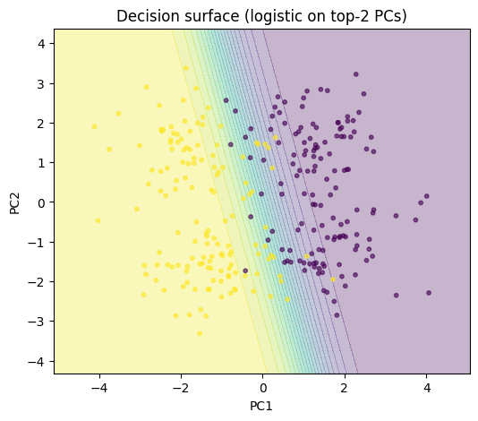

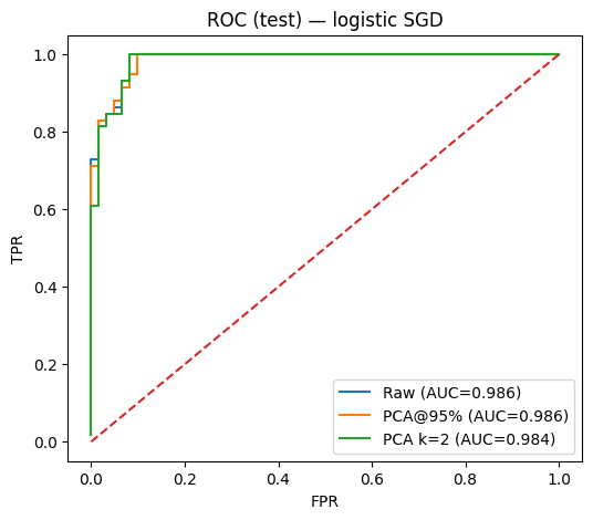
Plot: ROC curves (test set) — raw vs PCA

def roc_curve(scores, labels):
    scores = np.asarray(scores).ravel()
    labels = np.asarray(labels).astype(int).ravel()
    order = np.argsort(-scores, kind="mergesort")
    y = labels[order]
    P = y.sum()
    N = len(y) - P
    tps = np.cumsum(y)
    fps = np.cumsum(1 - y)
    tpr = tps / (P + 1e-12)
    fpr = fps / (N + 1e-12)
    return fpr, tpr


fpr_raw, tpr_raw = roc_curve(prob_raw, y_test)
fpr_95, tpr_95 = roc_curve(prob_pca95, y_test)
fpr_2, tpr_2 = roc_curve(prob_pca2, y_test)

plt.figure(figsize=(6, 5))
plt.plot(fpr_raw, tpr_raw, label=f"Raw (AUC={auc_raw:.3f})")
plt.plot(fpr_95, tpr_95, label=f"PCA@95% (AUC={auc_pca95:.3f})")
plt.plot(fpr_2, tpr_2, label=f"PCA k=2 (AUC={auc_pca2:.3f})")
plt.plot([0, 1], [0, 1], linestyle="--")
plt.xlabel("FPR")
plt.ylabel("TPR")
plt.title("ROC (test) — logistic SGD")
plt.legend()
plt.show()