Assignment: Empirical Evidence of Sparsity in High Dimensions (with PyTorch)

Goal. Use Monte Carlo experiments to show that, for a fixed number of samples (n), data become effectively “sparser” as the input dimension (d) grows.

Setup. For each (d {1,2,5,10,20,50,100}), draw (n) i.i.d. points (X_1,,X_n ([0,1]^d)).

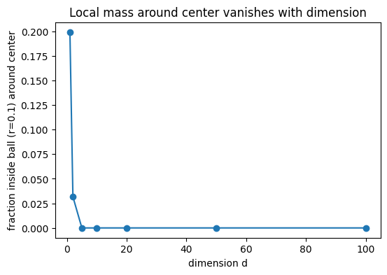
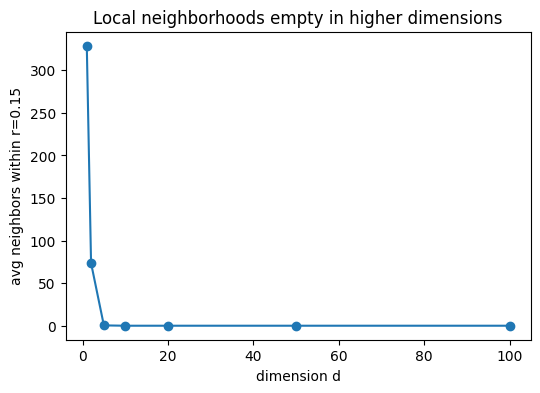
Tasks. 1. Nearest-neighbor distance grows. Compute the nearest-neighbor (NN) distance for each point and report the mean NN distance as a function of (d). Show that it increases with (d). 2. Distance concentration. Compute all pairwise Euclidean distances and report the coefficient of variation (std/mean). Show that the relative spread of distances shrinks with (d) (concentration of measure), making points nearly equidistant—hence no “close” neighbors. 3. Vanishing local mass. Fix a small radius (r>0) (e.g., (r=0.10)). Let (c=(0.5,,0.5)) be the hypercube center. Estimate the fraction of points within the ball (B(c,r)). Show it decreases with (d). 4. Local neighborhood empties. For a fixed small radius (r) (e.g., (r=0.15)), count how many neighbors each point has within that radius and report the average count vs (d). Show it decreases.

Deliverables. - A table with the metrics above for each (d). - Plots of (i) mean NN distance, (ii) coefficient of variation of pairwise distances, (iii) fraction inside (B(c,r)), (iv) average neighbor count within (r) — all vs (d).

Interpretation. Relate these observations to the curse of dimensionality. Explain how increased NN distances and distance concentration imply that models relying on local neighborhoods (e.g., kNN, kernels) struggle in high dimensions, and why uncertainty estimates (e.g., MLE variance) tend to inflate in sparse regions.

Setup

import torch
import math
import numpy as np
import pandas as pd
import matplotlib.pyplot as plt

torch.manual_seed(0)
print("PyTorch:", torch.__version__)

PyTorch: 2.7.1+cu126

Experiment parameters

# Dimensions to test and sample size
dims = [1, 2, 5, 10, 20, 50, 100]
n = 1200  # keep moderate; pairwise distances are O(n^2)

# Radii
r_center = 0.10  # fixed radius around center for Task 3
r_neighbors = 0.15  # fixed neighbor radius for Task 4

Helper functions

def pairwise_distances(x: torch.Tensor) -> torch.Tensor:
    """Compute Euclidean pairwise distances using torch.cdist.
    Args:
        x: (n, d) tensor
    Returns:
        (n, n) distance matrix
    """
    return torch.cdist(x, x)


def nearest_neighbor_distances(D: torch.Tensor) -> torch.Tensor:
    """Nearest-neighbor distance per point from a distance matrix.
    Args:
        D: (n, n) distance matrix
    Returns:
        (n,) tensor of NN distances
    """
    D_masked = D + torch.eye(D.size(0)) * 1e9
    nn_dist, _ = torch.min(D_masked, dim=1)
    return nn_dist

Run experiment and collect metrics

rows = []
for d in dims:
    # 1) Sample points in [0,1]^d
    X = torch.rand(n, d)

    # 2) Pairwise distances and NN stats
    D = pairwise_distances(X)
    tri = torch.triu_indices(n, n, offset=1)
    pdists = D[tri[0], tri[1]]
    pair_mean = pdists.mean().item()
    pair_std = pdists.std(unbiased=False).item()
    pair_cv = pair_std / (pair_mean + 1e-12)

    nn = nearest_neighbor_distances(D)
    mean_nn = nn.mean().item()
    median_nn = nn.median().item()

    # 3) Fraction inside ball around center
    center = torch.full((d,), 0.5)
    dist_to_center = torch.linalg.norm(X - center, dim=1)
    frac_in_ball = (dist_to_center <= r_center).float().mean().item()

    # 4) Average neighbors within fixed radius
    within = (D <= r_neighbors).float()
    within.fill_diagonal_(0.0)
    avg_neighbors = within.sum(dim=1).mean().item()

    rows.append(
        {
            "d": d,
            "mean_NN": mean_nn,
            "median_NN": median_nn,
            "pair_mean": pair_mean,
            "pair_std": pair_std,
            "pair_CV": pair_cv,
            f"frac_in_ball(r={r_center})": frac_in_ball,
            f"avg_neighbors(r={r_neighbors})": avg_neighbors,
            "n": n,
        }
    )

df = pd.DataFrame(rows)
df

	d	mean_NN	median_NN	pair_mean	pair_std	pair_CV	frac_in_ball(r=0.1)	avg_neighbors(r=0.15)	n
0	1	0.000402	0.000299	0.337809	0.238667	0.706515	0.199167	328.850006	1200
1	2	0.014385	0.013267	0.514249	0.244681	0.475803	0.031667	73.551666	1200
2	5	0.171974	0.171206	0.876517	0.248289	0.283267	0.000000	0.390000	1200
3	10	0.492865	0.494772	1.269582	0.245546	0.193407	0.000000	0.000000	1200
4	20	1.017114	1.018217	1.799921	0.243045	0.135031	0.000000	0.000000	1200
5	50	2.111619	2.115882	2.876143	0.241308	0.083900	0.000000	0.000000	1200
6	100	3.329890	3.332430	4.081142	0.239164	0.058602	0.000000	0.000000	1200

Save results to CSV

csv_path = "./high_dim_sparsity_metrics.csv"
df.to_csv(csv_path, index=False)
print("Saved:", csv_path)

Saved: ./high_dim_sparsity_metrics.csv

Plots

# 1) Mean NN distance vs d
plt.figure(figsize=(6, 4))
plt.plot(df["d"], df["mean_NN"], marker="o")
plt.xlabel("dimension d")
plt.ylabel("mean nearest-neighbor distance")
plt.title("Mean NN distance grows with dimension")
plt.show()

# 2) Coefficient of variation of pairwise distances vs d
plt.figure(figsize=(6, 4))
plt.plot(df["d"], df["pair_CV"], marker="o")
plt.xlabel("dimension d")
plt.ylabel("coeff. of variation of pairwise distances")
plt.title("Distance concentration (CV ↓) as dimension increases")
plt.show()

# 3) Fraction inside ball around center vs d
plt.figure(figsize=(6, 4))
plt.plot(df["d"], df[f"frac_in_ball(r={r_center})"], marker="o")
plt.xlabel("dimension d")
plt.ylabel(f"fraction inside ball (r={r_center}) around center")
plt.title("Local mass around center vanishes with dimension")
plt.show()

# 4) Average #neighbors within fixed radius vs d
plt.figure(figsize=(6, 4))
plt.plot(df["d"], df[f"avg_neighbors(r={r_neighbors})"], marker="o")
plt.xlabel("dimension d")
plt.ylabel(f"avg neighbors within r={r_neighbors}")
plt.title("Local neighborhoods empty in higher dimensions")
plt.show()

Interpretation

Nearest neighbors recede: The mean nearest-neighbor distance grows with (d), so “local” neighborhoods become larger in absolute terms.
Distances concentrate: The coefficient of variation (std/mean) of pairwise distances shrinks as (d) increases, so most pairs are at similar distances—no truly “close” neighbors.
Vanishing local mass: The fraction of samples in a fixed-radius ball around the center tends to 0 with increasing (d).
Empty neighborhoods: With a fixed small radius, the average number of neighbors within that radius drops steeply as (d) grows.

These effects illustrate the curse of dimensionality: methods reliant on local neighborhoods (kNN, kernels) become data-hungry; likewise, uncertainty estimates (e.g., MLE variance) inflate away from the rare dense pockets of data.