Regression tree stumps#
A regression tree stump is a tree with a decision node at the root and two predictor leaves. The leaves predict the average of the target values held by that leaf, assuming we are minimizing the mean squared error (MSE) loss function.
To keep things simple, this example assumes that only a single predictor variable, \(x\), is associated with the target variable, \(y\).
from sklearn.metrics import mean_squared_error
from sklearn.tree import DecisionTreeRegressor
import matplotlib.pyplot as plt
from dtreeviz.trees import *
from lolviz import *

import numpy as np
import pandas as pd
Define decision and leaf nodes and how to predict#
Because decision and predictor nodes have different behavior, it makes sense to create two different classes. To make a prediction for test vector \(X\), a decision node compares the predictor variable (feature) \(x_i\) against a split value. (We only have one predictor here so we don’t bother recording which feature a node is testing.) The split value will be chosen from the range of \(x_i\) during training (see below).
class DecisionNode:
    def __init__(self,split): # split chosen from x values
        self.split = split
    def predict(self,x):
        if x < self.split:
            return self.left.predict(x)
        return self.right.predict(x)

class LeafNode:
    def __init__(self,y,left=None,right=None):
        self.y = y
    def predict(self, x): # Predictions are the means of subregions (x ignored in leaf)
        return np.mean(self.y)
Given these definitions, let’s manually build a stump and make a prediction or two.
root = DecisionNode(900)                 # split on x at 900
root.left = LeafNode([1160, 1200, 1280]) # 3 y values in leaf
root.right = LeafNode([1450,2000])

x = 900
y_pred = root.predict(x)
print(f"{x} => {y_pred:.1f} (avg [1450,2000] is {np.mean([1450,2000])})")

x = 890
y_pred = root.predict(x)
print(f"{x} => {y_pred:.1f} (avg [1450,2000] is {np.mean([1450,2000])})")
900 => 1725.0 (avg [1450,2000] is 1725.0)
890 => 1213.3 (avg [1450,2000] is 1725.0)
Fit a stump to single-var x and target y#
def fit(x, y):
    """
    We train on the (x,y), getting split of single-var x that
    minimizes variance in subregions of y created by x split.
    Return root of decision tree stump
    """
    loss, split = find_best_split(x,y)
    root = DecisionNode(split)
    root.left = LeafNode(y[x<split])
    root.right = LeafNode(y[x>=split])
    return root

def find_best_split(x,y):
    best_loss = np.inf
    best_split = -1
    print(f"find_best_split in x={list(x)}")
    for v in x[1:]: # try all possible x values
        lefty = y[x<v].values
        righty = y[x>=v].values
        nl = len(lefty)
        nr = len(righty)
        if nl==0 or nr==0:
            continue
        # variance is same as MSE here
        # weight by proportion on left and right, get avg as loss
        loss = (np.var(lefty)*nl + np.var(righty)*nr)/2
        print(f"{lefty} | {righty}    candidate split x ={v:4d} loss {loss:8.1f}")
        if loss < best_loss:
            best_loss = loss
            best_split = v
    return float(best_loss), best_split
Use data from explained.ai article#
Grabbed trivial data from Gradient boosting: Distance to target:
df = pd.DataFrame()
df["sqfeet"] = [750, 800, 850, 900,950]
df["rent"] = [1160, 1200, 1280, 1450,2000]
df
| sqfeet | rent | |
|---|---|---|
| 0 | 750 | 1160 |
| 1 | 800 | 1200 |
| 2 | 850 | 1280 |
| 3 | 900 | 1450 |
| 4 | 950 | 2000 |
t = fit(df.sqfeet, df.rent)
find_best_split in x=[750, 800, 850, 900, 950]
[1160] | [1200 1280 1450 2000]    candidate split x = 800 loss 194837.5
[1160 1200] | [1280 1450 2000]    candidate split x = 850 loss 142033.3
[1160 1200 1280] | [1450 2000]    candidate split x = 900 loss  79358.3
[1160 1200 1280 1450] | [2000]    candidate split x = 950 loss  24737.5
Visualize tree with lolviz#
See lolviz
treeviz(t)

Tweak last rent price to bring inline#
We get a different split
df = pd.DataFrame()
df["sqfeet"] = [750, 800, 850, 900,950]
df["rent"] = [1160, 1200, 1280, 1450,1300]
df
| sqfeet | rent | |
|---|---|---|
| 0 | 750 | 1160 |
| 1 | 800 | 1200 |
| 2 | 850 | 1280 |
| 3 | 900 | 1450 |
| 4 | 950 | 1300 |
t = fit(df.sqfeet, df.rent)
treeviz(t)
find_best_split in x=[750, 800, 850, 900, 950]
[1160] | [1200 1280 1450 1300]    candidate split x = 800 loss  16337.5
[1160 1200] | [1280 1450 1300]    candidate split x = 850 loss   9033.3
[1160 1200 1280] | [1450 1300]    candidate split x = 900 loss   9358.3
[1160 1200 1280 1450] | [1300]    candidate split x = 950 loss  24737.5

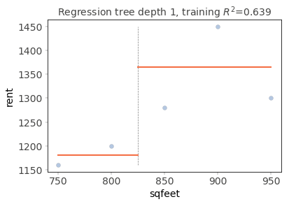
Visual partitioning of stump via dtreeviz#
See dtreeviz.
fig = plt.figure()
ax = fig.gca()
X, y = df.sqfeet, df.rent
t = rtreeviz_univar(ax,
                    X, y,
                    max_depth=1,
                    feature_name='sqfeet',
                    target_name='rent',
                    fontsize=14)
plt.show()
Visual partitioning of stump nodes#
regr = DecisionTreeRegressor(max_depth=1)

X, y = df.sqfeet.values.reshape(-1,1), df.rent
regr = regr.fit(X, y)
viz = dtreeviz(regr, X, y, target_name='rent',
               feature_names=['sqfeet'],
               fancy=True)
#viz.view() # to pop up outside of notebook
viz
/Users/parrt/anaconda3/lib/python3.7/site-packages/matplotlib/tight_layout.py:176: UserWarning: Tight layout not applied. The left and right margins cannot be made large enough to accommodate all axes decorations.
  warnings.warn('Tight layout not applied. The left and right margins '

Full regression tree fit#
def fit(x, y):
    """
    We train on the (x,y), getting split of single-var x that
    minimizes variance in subregions of y created by x split.
    Return root of decision tree stump
    """
    if len(x)==1:
        return LeafNode(y)
    loss, split = find_best_split(x,y)
    if split==-1:
        return LeafNode(y)
    t = DecisionNode(split)
    left = x[x<split]
    right = x[x>=split]
    t.left = fit(left, y[x<split])
    t.right = fit(right, y[x>=split])
    return t
df = pd.DataFrame()
df["x"] = [700, 100, 200, 600, 800]
df["y"] = [10, 2, 3, 11, 9]
df
| x | y | |
|---|---|---|
| 0 | 700 | 10 |
| 1 | 100 | 2 |
| 2 | 200 | 3 |
| 3 | 600 | 11 |
| 4 | 800 | 9 |
t = fit(df.x, df.y)
treeviz(t)
find_best_split in x=[700, 100, 200, 600, 800]
[2] | [10  3 11  9]    candidate split x = 200 loss     19.4
[2 3] | [10 11  9]    candidate split x = 600 loss      1.2
[10  2  3 11] | [9]    candidate split x = 800 loss     32.5
find_best_split in x=[100, 200]
[2] | [3]    candidate split x = 200 loss      0.0
find_best_split in x=[700, 600, 800]
[10 11] | [9]    candidate split x = 800 loss      0.2
find_best_split in x=[700, 600]
