Adaptive Boosting (AdaBoost)

In this chapter we are treating adaptive boosting that uses ensembles of many weak learner, to produce a stronger learner. In contrast to other ensemble methods though such as random forests, boosting methods, train predictors sequentially rather than parallel.

If we imagine a sequence of weak learners like in random forests, boosting starts with training the first learner and at each subsequent step, due to its sequential nature, it considers the mistakes of the preceding learning step as shown below.

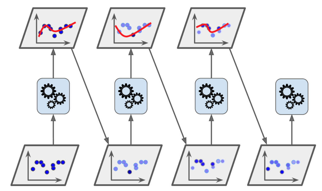Boosting methods act sequentially considering the prediction results of the preceding learners.

Lets see how AdaBoost functions using an example based on this article.

Lets assume that you are a data scientist working on a dating site and you are asked to develop an algorithm that classifies whether a profile is attractive or not. The dataset you are given is shown below. This is of course a fictitious dataset - there is no way that someone will put in their profile that they are not smart or polite.

\[\mathtt{data} = \{ (\mathbf{x}_1, y_1), \dots, (\mathbf{x}_m, y_m) \}\]

Weight	Smart	Polite	Fit	Attractive
180	no	no	no	no
150	yes	yes	no	no
175	no	yes	yes	yes
165	yes	yes	yes	yes
190	no	yes	no	no
201	yes	yes	yes	yes
185	yes	yes	no	yes
168	yes	no	yes	yes

We assume that the label \(y \in {+1, -1}\) instead of 0 or 1 with loss of generality. This is a binary classification problem but the method is equally applicable to multi-class problems.

AdaBoost calls a given weak learner repeatedly in a series of rounds \(t=1, \dots, T\), each weak learner is denoted by \(h_t\) - the weak hypothesis that each learner evaluates. In this example case, we can elect a hypothesis set from the family of decision trees and the specific hypothesis we will use is a decision tree with single split (depth = 1) called decision stump.

One of the main ideas of the AdaBoost is to maintain a distribution of weights over the training set. In each round, the weights of incorrectly classified examples are increased so that the weak learner is forced to focus on the hard examples in the training set. The size of the weight vector equals \(m\), the number of examples we are given. The weight of training example \(i\) on round \(t\) is denoted \(w_t(i)\).

Initially, all weights are set equally,

\[w_0(i)=\frac{1}{m}\]

At each round \(t\) we have \(n\) decision stumps each producing \(\hat{\mathbf y}_t\) decisions. We need to find which stump best fits the examples, we can try every feature of the input along with every possible threshold and see which one offers the lower error rate. We therefore compare the predictions made by each weak learner with the actual labels in the training set to produce the weighted error rate \(\epsilon_t\)

\[\epsilon_t = \Pr [\hat y_t(i) \neq y_t(i)] = \frac{\sum_{i: \hat y_t(i) \neq y_t(i)}^m w_t(i)}{\sum_{i=1}^m w_t(i)}\]

The decision stump that offers the lower error rate, has a much higher significance given via the formula

\[\alpha_t = \eta \log \frac{1-\epsilon_t}{ϵ_t}\]

where \(\eta\) is a learning rate hyperparameter - if not optimized it defaults to 1.0.

Then AdaBoost updates the example weights via the equations below that boosts the weights of misclassified examples and normalizes them so that they can be interpreted as a probability distribution:

\[\begin{split}w_t(i) = \begin{cases}w_t(i) & \text{if }\hat y_t(i) = y_t(i), \\ w_t(i) \exp(\alpha_t) & \text{if } \hat y_t(i) \neq y_t(i) \end{cases}\end{split}\]

\[w_t(i) = \frac{w_t(i)}{\sum_{=1}^m w_t(i)}\]

The process is repeated in the next round with each round determining a weak hypothesis. At the end we make the final hypothesis

\[\hat y (\mathbf x) = \sum_{t=1}^T \alpha_t h_t(\mathbf x)\]

which can be interpreted as the weighted majority vote of the T weak hypotheses. As shown in the figure below for various values of \(\eta\),

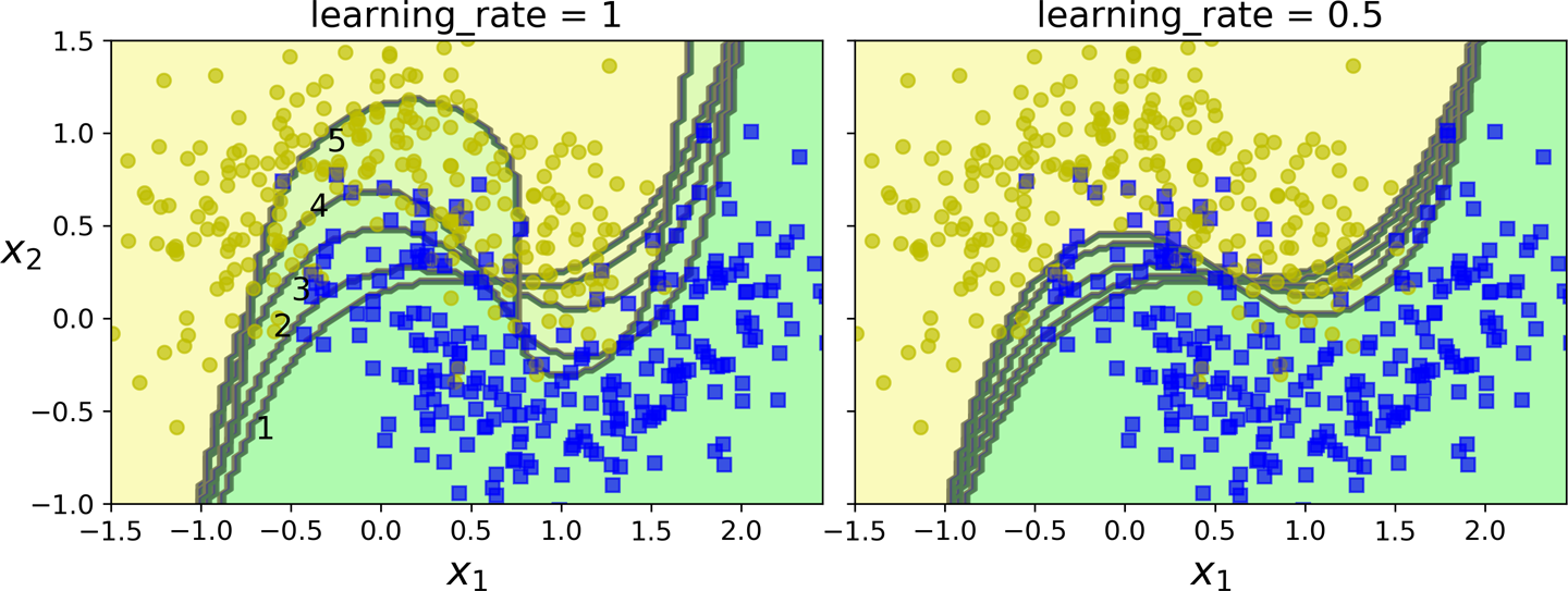The first classifier gets many instances wrong, so their weights get boosted. The second classifier therefore does a better job on these instances, and so on. The plot on the right represents the same sequence of predictors, except that the learning rate is halved (i.e., the misclassified instance weights are boosted half as much at every iteration). As you can see, this sequential learning technique has some similarities with Gradient Descent, except that instead of tweaking a single predictor’s parameters to minimize a cost function, AdaBoost adds predictors to the ensemble, gradually making it better.

A perhaps more illuminating example that shows the weight adjustments is shown below. You need to replace the \(m\) with \(t\) to match the notation of these notes.

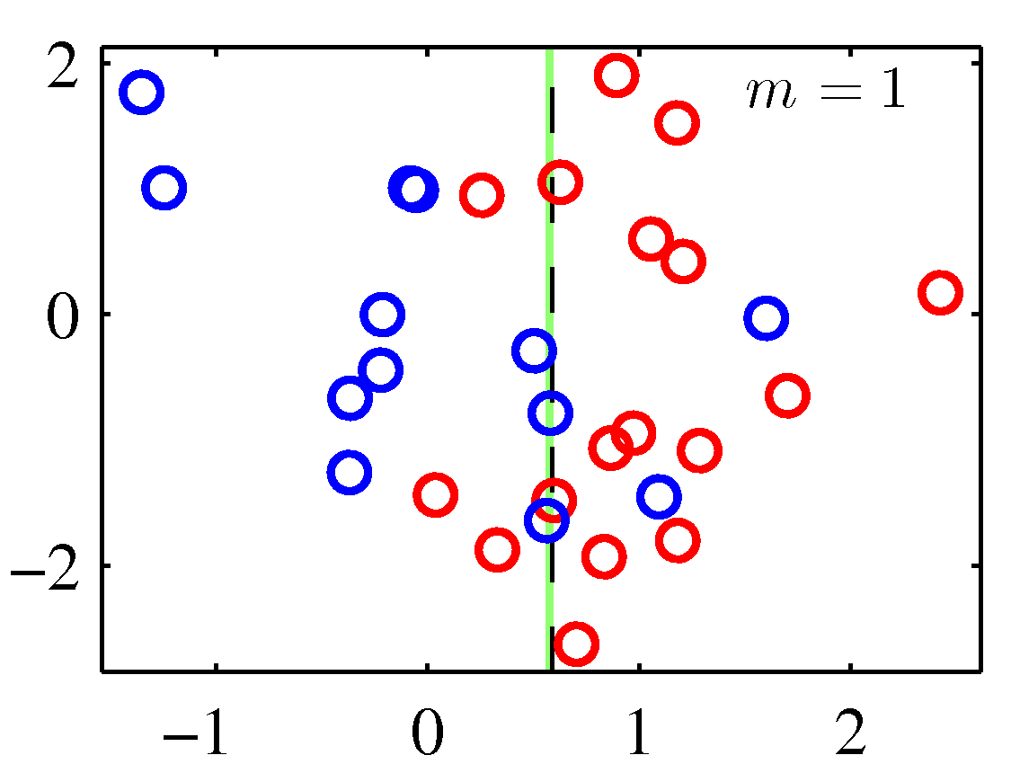
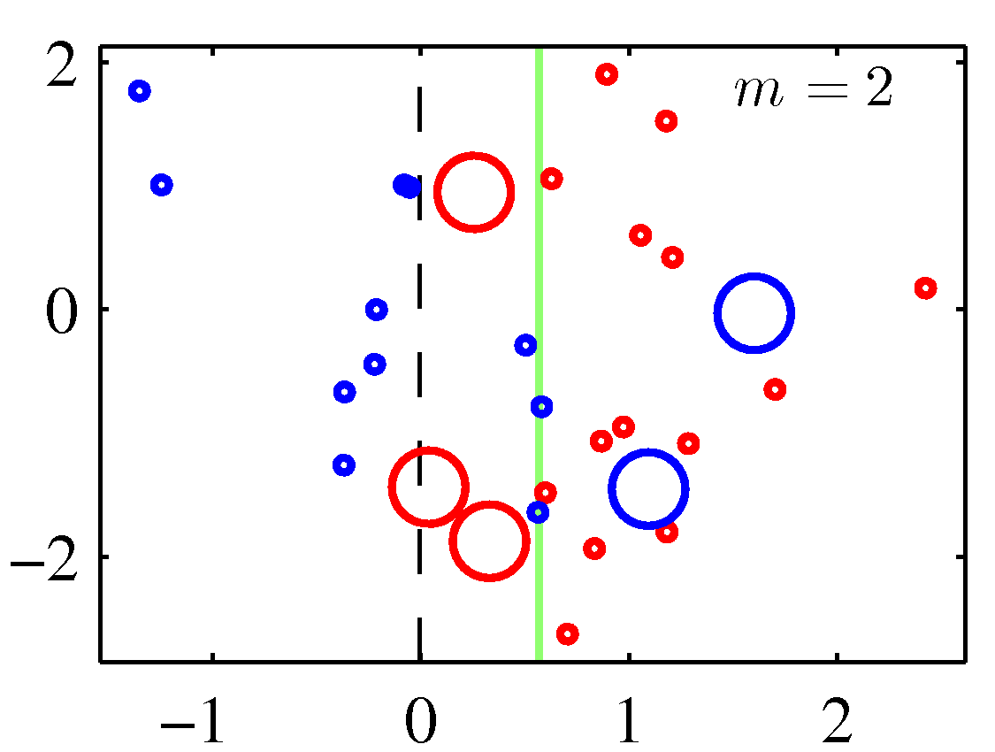
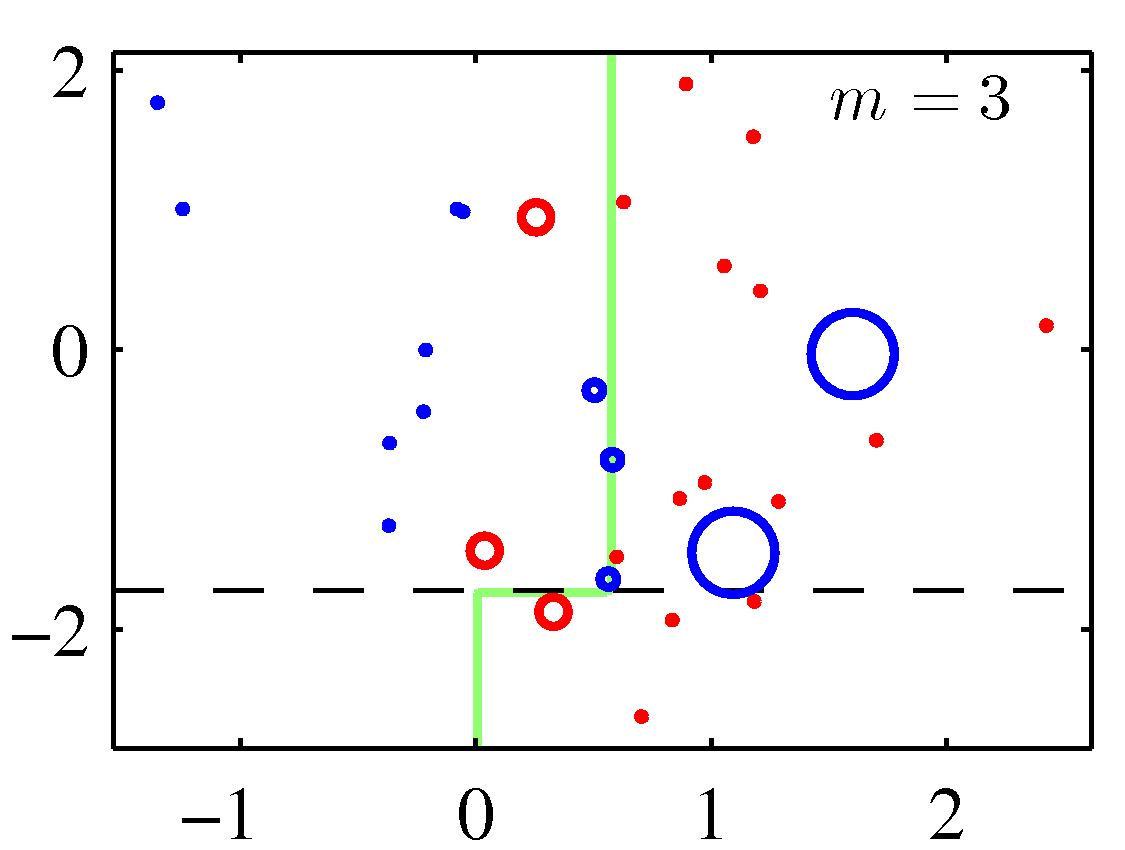
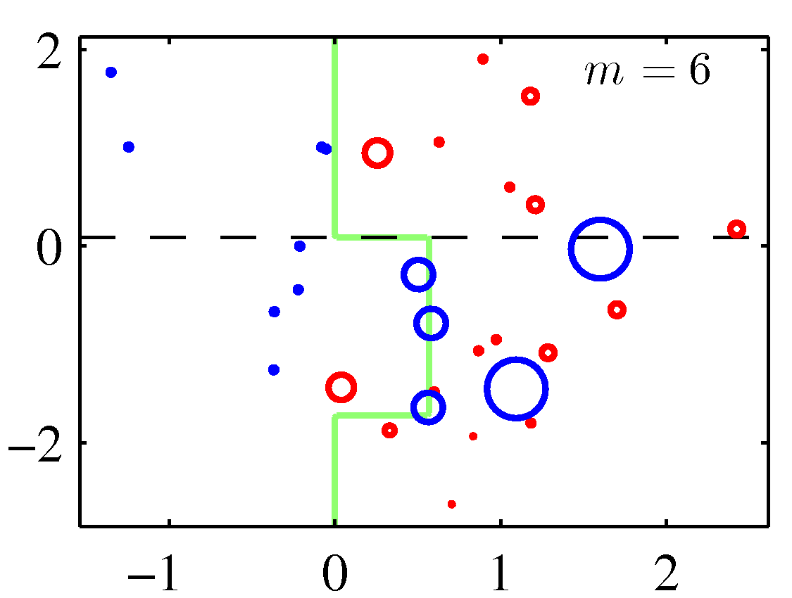
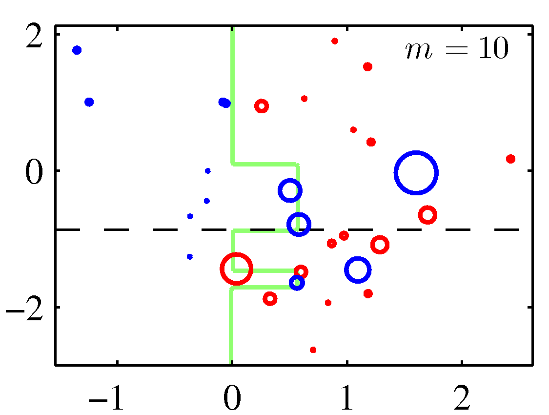
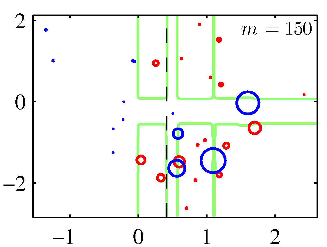
Note that although decision stumps were used to produce the adaboost decision boundaries above, the method is generic to any weak learner. Also note that there weights for the correctly classified data points are decreased in these figures instead of keeping them constant. Either of the two options should perform similarly.