The Netflix Prize and Singular Value Decomposition #
NOTE: The following are based on the winning submission paper as well as their subsequent publication.
Problem Statement #
The Netflix Prize was an open competition for the best collaborative filtering algorithm to predict user ratings for films, based on previous ratings without any other information about the users or films, i.e. without the users or the films being identified except by numbers assigned for the contest.
The competition was held by Netflix, and on September 21, 2009, the grand prize of US $1,000,000 was given to the BellKor’s Pragmatic Chaos team which bested Netflix’s own algorithm for predicting ratings by 10.06%
This competition is instructive since:
-
Collaborative filtering models try to capture the interactions between users and items that produce the different rating values. However, many of the observed rating values are due to effects associated with either users or items, independently of their interaction. A prime example is that typical CF data exhibit large user and item biases – i.e., systematic tendencies for some users to give higher ratings than others, and for some items to receive higher ratings than others.
-
Observing the posted improvements in RMSE over time, the competition has become of little business value to Netflix after a while. This means that it was unlikely that any minute improvement to RMSE (e.g. 0.1%) will translate to additional revenue.
-
The 10% improvement goal was a lucky number after all. Netflix had no clue as to if this was the right number when they defined the terms. Any small deviation from this number, would have made the competition either too easy or impossibly difficult.
You are given the following dataset structure (will be explained in class) shown below,
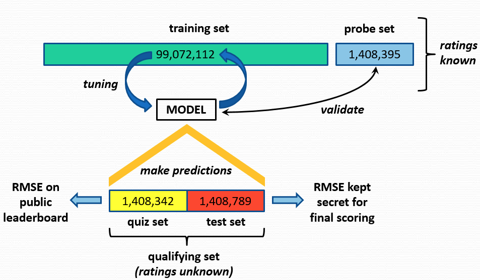 Netflix Prize dataset structure
Assuming that the rating matrix $A_{[m x n]}$ with m users (500K) and n items (17K movies), this matrix is extremely sparse - it has only 100 million ratings, the remaining 8.4 billion ratings are missing (about 99% of the possible ratings are missing, because a user typically rates only a small portion of the movies).
SVD Solution #
Given the very large data matrix it was only expected that competitors attempted to do dimensionality reduction and as it turns out this was the basis for the winning algorithm. Dimensionality reduction can be done via matrix factorization that has the following advantage: when explicit feedback is not available, we can infer user preferences using implicit feedback, which indirectly reflects opinion by observing user behavior including purchase history, browsing history, search patterns, or even mouse movements. A high level visual result of the matrix factorization with two latent features is shown below:
 Simplistic illustration of two latent factor approach. Users and Items are shown in this feature space.
Lets now look at one matrix factorization method in detail, recalling the premise of SVD from linear algebra: it is a decomposition that can work with rectangular matrices and can result into a factorization:
$$A = U \Sigma V^†$$
where $\mathbf{U}$ is a $m \times m$ real unitary matrix, $\mathbf{\Sigma}$ is an $m \times n$ rectangular diagonal matrix with non-negative real numbers on the diagonal, and $\mathbf{V}$ is a $n \times n$ real unitary matrix.
Remember that a unitary matrix $U$ is a matrix that its conjugate transpose $U^†$ is also its inverse - its the complex analog of the orthogonal matrix and we have by definition $UU^†=I$.
The columns of $U$ are eigenvectors of $AA^T$, and the columns of $V$ are eigenvectors of $A^TA$. The $r$ singular values on the diagonal of $\Sigma$ are the square roots of the nonzero eigenvalues of both $AA^T$ and $A^TA$.
It is interesting to attribute the columns of these matrices with the four fundamental subspaces:
- The column space of $A$ is spanned by the first $r$ columns of $U$.
- The left nullspace of $A$ are the last $m-r$ columns of $U$.
- The row space of $A$ are the first $r$ columns of $V$.
- The nullspace of $A$ are the last $n-r$ columns of V.
We can write the SVD as,
$$A = U \sqrt{\Sigma} \sqrt{\Sigma} V^†$$
and given the span of the subspaces above we can now intuitively think what the terms $\mathbf{p}_u = U \sqrt{\Sigma}$ and $\mathbf{q}_i = \sqrt{\Sigma} V^†$ represent.
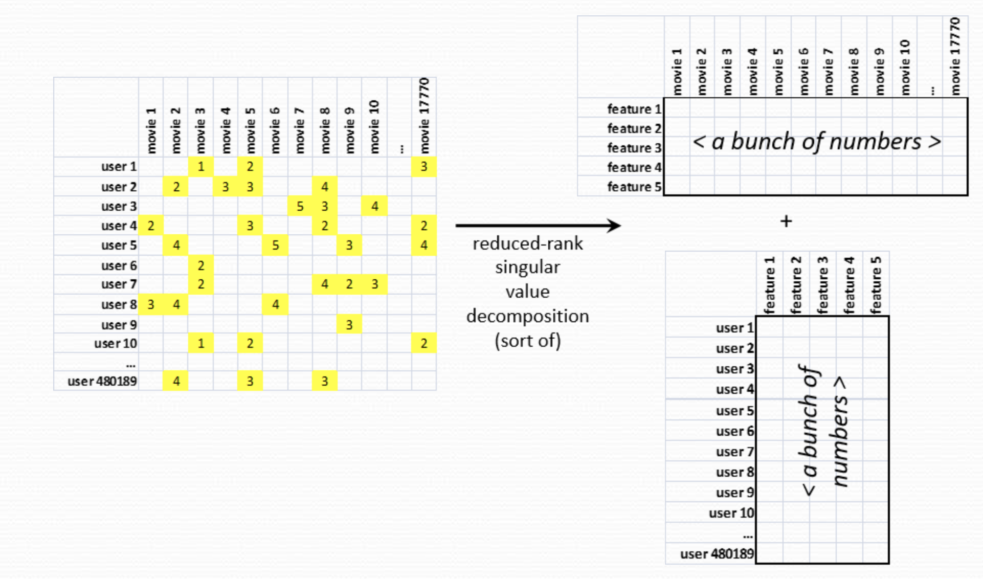 SVD decomposition reveals latent features weighted by the underlying singular values of the data matrix
The first term represents the column space and it provides a representation of all inter-user factors (also called latent (hidden) features). The second term represents the row space and it provides a representation of all inter-item factors. Which brings us to the major point of what the $\sqrt{\Sigma}$ is doing to both terms. It represents the significance of those factors and therefore we can very easily use the singular values it contains to “compress” our representation by selecting the $f$ largest singular values and ignoring the rest.
Given these vectors of factors we can now use them to predict the rating:
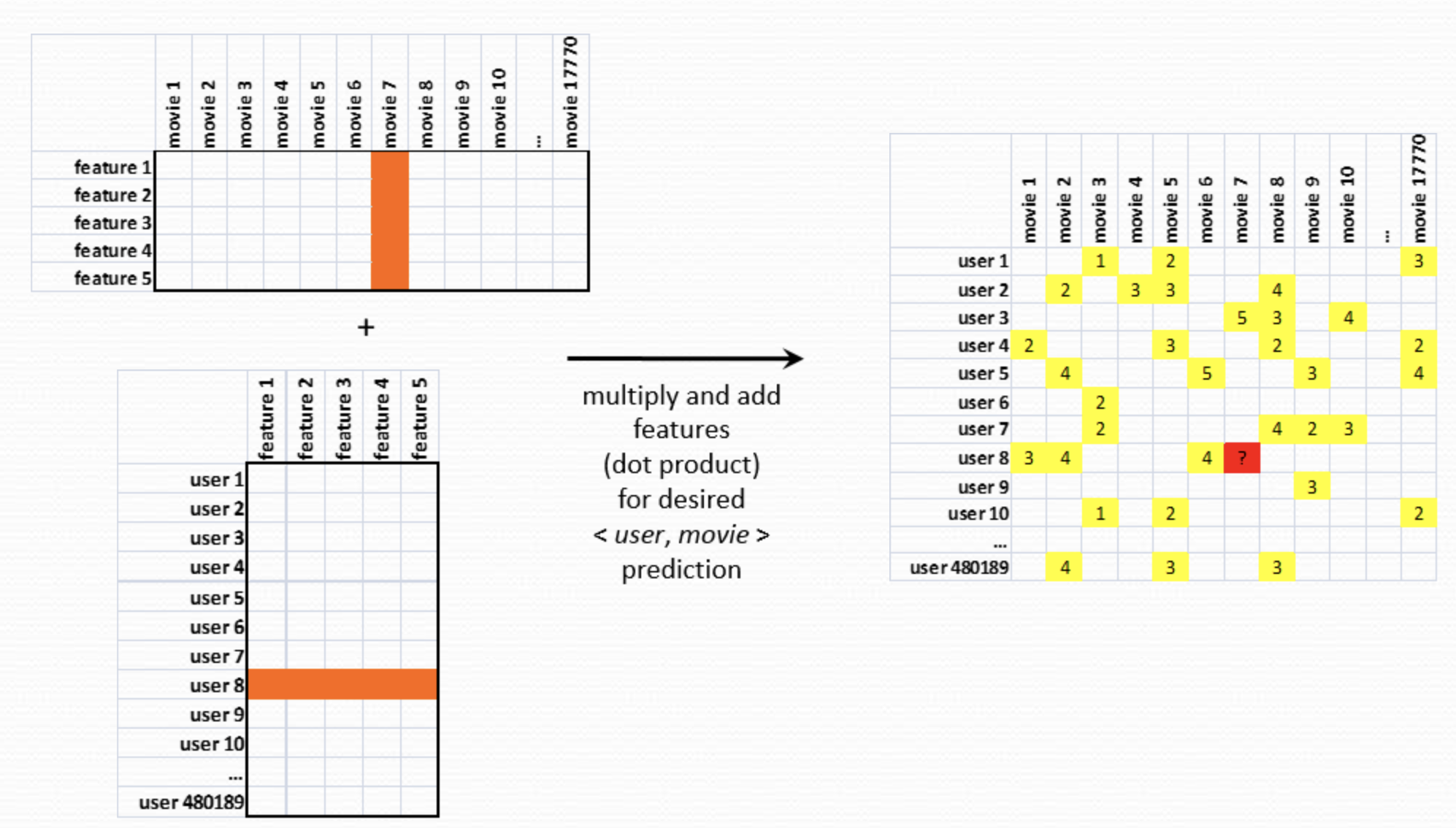 Prediction of a rating is the product between user latent features and movie latent features matrices.
We have seen above graphically how the matrix factorization models map both users and items to a joint latent factor space of dimensionality $f$, such that user-item interactions are modeled as inner products in that space. Each item $i$ is associated with a vector $q_i \in \mathbb{R}^f$, and each user $u$ is associated with a vector $p_u \in \mathbb{R}^f$. For a given item $i$, the elements of $q_i$ measure the extent to which the item possesses those factors, positive or negative. For a given user $u$, the elements of $p_u$ measure the extent of interest the user has in items that are high on the corresponding factors, again, positive or negative. The resulting dot product, $q_i^T p_u$, captures the interaction between user $u$ and item $i$ — the user’s overall interest in the item’s characteristics. This approximates user $u$’s rating of item $i$, which is denoted by $r_{ui}$, leading to the estimate
$$\hat{r}_{ui}= q_i^T p_u$$
The major challenge is computing the mapping of each item and user to factor vectors $q_i$, $p_u$. After the recommender system completes this mapping, it can easily estimate the rating a user will give to any item by the above equation.
Obvious a standard SVD decomposition is not defined for sparse matrices that we have in practice ($mxn$) so we can estimate the factors $q_i$ and $p_u$ using the following objective function that is based on minimizing the mean squared error (MSE) between the actual rating and the estimate,
$$ \min_{p, q} \sum_{(u, i) \in \kappa} (r_{ui} - q_i^T p_u)^2 + \lambda (||q_i||^2 + ||p_u||^2)$$
where $κ$ is the set of the $(u,i)$ pairs for which $r_{ui}$ is known (the training set).
The system learns the model by fitting the previously observed ratings. However, the goal is to generalize those previous ratings in a way that predicts future, unknown ratings. Thus, the system should avoid over-fitting the observed data by regularizing the learned parameters using their squared magnitude and the hyperparameter $\lambda$.
We can solve this minimization problem using the well known Stochastic Gradient Descent (SGD) method. Simon Funk popularized a stochastic gradient descent optimization wherein the algorithm loops through all ratings in the training set. For each given training case, the system predicts $r_{ui}$ and computes the associated prediction error
$$e_{ui}=r_{ui}-q_i^T p_u$$
Then it modifies the parameters by a magnitude proportional to $\gamma$ in the opposite direction of the gradient, combines implementation ease with a relatively fast running time:
$$q_i \leftarrow q_i + \gamma (e_{ui}p_u - \lambda q_i) $$ $$p_u \leftarrow p_u + \gamma (e_{ui}q_i - \lambda p_u) $$
Iterating, we can estimate the final factors we are after and insert predictions in our stream when the user launches the Netflix app.